编程模型和语言层

import transform.TpuLang as tpul

tpul.init("BM1684X", True)

# 定义输入
x = tpul.Tensor(dtype="float32", shape=[1, 3, 224, 224], name="input")

# 添加自定义算子
def shape_func(tensors_in):
    return [tensors_in[0].shape]

outs = tpul.custom(
    tensors_in=[x],
    shape_func=shape_func,
    op_name="custom_op_name",
    params={"param1": value1, "param2": value2},
    out_dtypes=["float32"],
    out_names=["custom_out"]
)

# 编译生成 MLIR
tpul.compile("model_name", [x], outs, False, 2, has_custom=True)

2. 后端实现

在 $TPUC_ROOT/customlayer/include 添加头文件。
在 $TPUC_ROOT/customlayer/src 添加实现文件。
在 backend_custom_param.h 定义参数结构体。
添加 API 接口文件。
在 backend_custom_api.cpp 定义后端调用接口。
运行 $TPUC_ROOT/customlayer/build.sh 编译生成动态库。

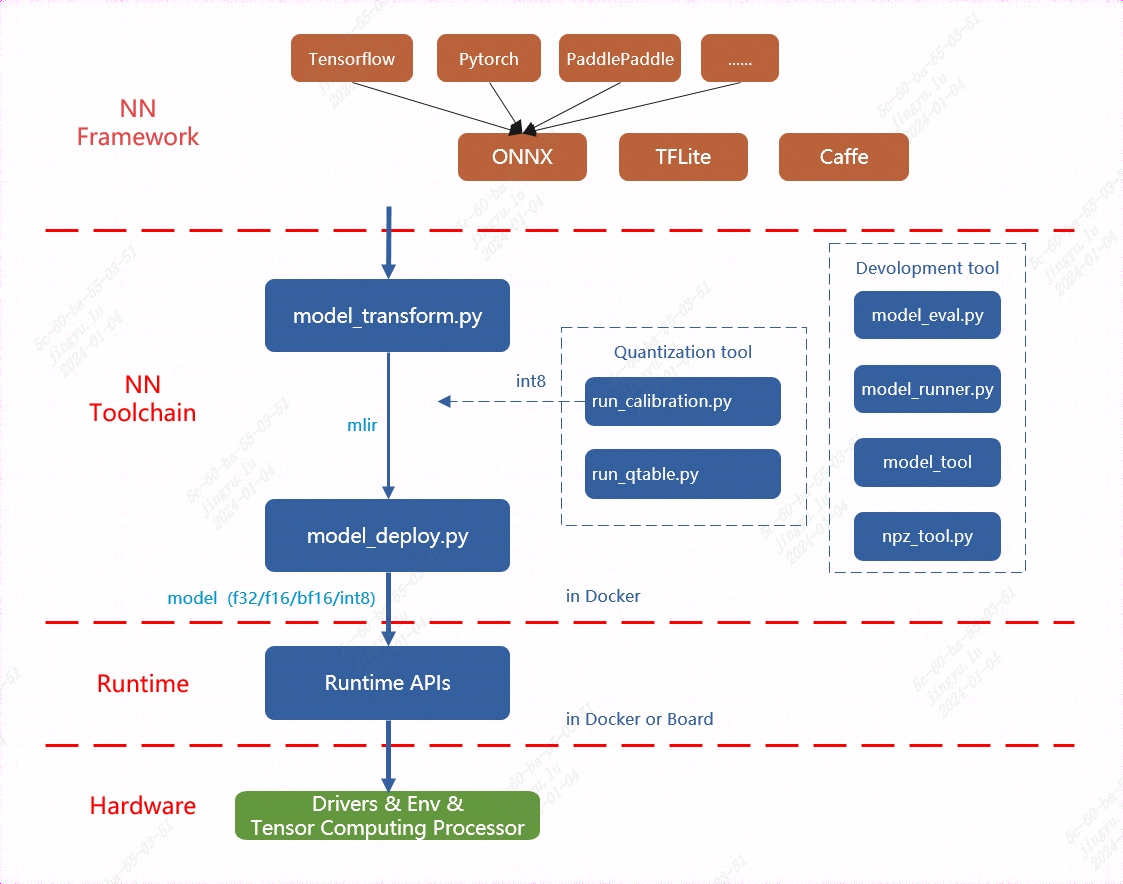
TPU-MLIR 提供了一个强大的工具链，支持从多种深度学习框架到 TPU 可执行模型的转换。通过支持自定义算子，它为开发者提供了极大的灵活性，使得复杂的深度学习模型能够在 TPU 上高效运行。结合 TPUPerf 工具，开发者可以全面优化和验证其模型性能。 TPU平台专门支持BModel模型加速，因此在使用TPU之前，必须进行模型迁移。通过利用MLIR工具链，可以将在其他框架中训练的模型转换为BModel，从而实现TPU的兼容运行。 MLIR已经直接支持绝大多数开源框架（如Pytorch、ONNX、TFLite和Caffe）中的算子和模型，而对于其他框架（如TensorFlow和PaddlePaddle），则需要先将其转换为ONNX模型，然后再进行后续转换。这一过程的整体架构可以参见TPU-MLIR工具链示意图。 alt text 模型转换主要包括两个步骤。首先，通过 model_transform.py 脚本将原始模型转换为 MLIR 文件。然后，使用 model_deploy.py 脚本将生成的 MLIR 文件转换为 BModel。

在生成浮点型模型时，model_deploy.py 工具支持输出三种不同的浮点数据类型：F32、F16 和 BF16。而对于 INT8 模型，首先需要准备一个量化数据集，并调用 run_calibration.py 生成校准表。接着，将校准表传递给 model_deploy.py 以完成 INT8 模型的生成。

如果生成的 INT8 模型精度不符合要求，可以使用 run_qtable.py 工具生成量化表，量化表用于决定哪些网络层使用浮点计算，随后将该量化表传递给 model_deploy.py，以生成混合精度模型。

以 yolov5s.onnx 为例, 介绍如何编译迁移一个onnx模型至BM1684X 平台运行。

在与 tpu-mlir 同级的目录下创建一个名为 model_yolov5s 的目录，并将模型文件和图片文件都放入该目录。具体步骤如下：

进入正确的父目录**：确保位于与 tpu-mlir 同级的目录中。例如：
```
cd /path/to/your/parent_directory
```
创建 model_yolov5s 目录：
```
mkdir model_yolov5s
```
将模型文件和COCO2017数据集图片文件复制到新建的 model_yolov5s 目录中：
```
cp /path/to/your/model_file /path/to/your/image_file ./model_yolov5s/
```
确保将模型文件（例如 .pt、.onnx、.mlir 等格式的文件）和图片文件（例如 .jpg、.png 等格式的图片）都放入 model_yolov5s 目录中。完成后，目录结构应该类似于以下形式：

/parent_directory
  ├── tpu-mlir
  └── model_yolov5s
      ├── your_model_file
      └── your_image_file

如果模型的输入是图片格式，在进行模型转换前，必须先了解并执行必要的预处理操作。然而，如果模型输入的是已经经过预处理的 npz 文件，则无需再进行额外的预处理步骤。在官方的 YOLOv5 模型中，图片输入采用 RGB 格式，并且每个像素值都会乘以 1/255 进行归一化处理。这相当于将每个像素的值缩放至 0 到 1 之间。对应地，转换时的 mean（均值）为 [0.0, 0.0, 0.0]，而 scale（缩放系数）为 [0.0039216, 0.0039216, 0.0039216]，因为 1/255 等于 0.0039216。模型转换命令如下:

$ model_transform.py \
    --model_name yolov5s \
    --model_def ../yolov5s.onnx \
    --input_shapes [[1,3,640,640]] \
    --mean 0.0,0.0,0.0 \
    --scale 0.0039216,0.0039216,0.0039216 \
    --keep_aspect_ratio \
    --pixel_format rgb \
    --output_names 350,498,646 \
    --test_input ../image/dog.jpg \
    --test_result yolov5s_top_outputs.npz \
    --mlir yolov5s.mlir

在模型转换为 MLIR 文件后，会生成一个名为 ${model_name}_in_f32.npz 的文件。该文件包含模型的输入数据，以 .npz 格式存储，通常用于模型推理时作为输入文件，确保数据格式与模型的输入要求一致。将 MLIR 文件转换为 F32 格式的 BModel，操作步骤如下：

$ model_deploy.py \
     --mlir yolov5s.mlir \
     --quantize F32 \
     --chip bm1684x \
     --test_input yolov5s_in_f32.npz \
     --test_reference yolov5s_top_outputs.npz \
     --tolerance 0.99,0.99 \
     --model yolov5s_1684x_f32.bmodel

编译完成后, 会生成名为 yolov5s_1684x_f32.bmodel 的文件。将 MLIR 文件转换为 F16 格式的 BModel，具体操作步骤如下：

$ model_deploy.py \
    --mlir yolov5s.mlir \
    --quantize F16 \
    --chip bm1684x \
    --test_input yolov5s_in_f32.npz \
    --test_reference yolov5s_top_outputs.npz \
    --model yolov5s_1684x_f16.bmodel

编译完成后, 会生成名为 yolov5s_1684x_f16.bmodel 的文件。在转换为 INT8 模型之前，首先需要运行校准过程（calibration）来生成校准表。校准过程中，输入的数据数量根据具体需求准备，通常在 100 到 1000 张图片左右。

生成校准表后，可以选择生成对称或非对称的 BModel。如果对称模型能满足需求，通常不建议使用非对称模型，因为非对称模型的性能会稍逊于对称模型。

以下是使用现有的 100 张来自 COCO2017 数据集的图片作为示例，执行校准的步骤：

准备校准数据集：确保已经准备好 100 张 COCO2017 的图片，并将其放置在指定的目录中。
运行校准命令：通过以下命令运行校准，生成校准表：

$ run_calibration.py yolov5s.mlir \
    --dataset ../COCO2017 \
    --input_num 100 \
    -o yolov5s_cali_table

生成 INT8 模型：使用生成的校准表，执行以下命令，将校准表传递给 model_deploy.py 以生成对称或非对称的 INT8 BModel：

$ model_deploy.py \
    --mlir yolov5s.mlir \
    --quantize INT8 \
    --calibration_table yolov5s_cali_table \
    --chip bm1684x \
    --test_input yolov5s_in_f32.npz \
    --test_reference yolov5s_top_outputs.npz \
    --tolerance 0.85,0.45 \
    --model yolov5s_1684x_int8_sym.bmodel

如果对称模型能够满足精度要求，通常选择对称模式，因为它的性能表现优于非对称模型。编译完成后, 会生成名为 yolov5s_1684x_int8_sym.bmodel 的文件。

效果检验

完成目标检测的整个流程，包括数据预处理、推理、后处理（NMS）和结果的可视化。

图像预处理：将输入图像缩放到模型接受的尺寸。
推理：调用 mlir_inference 或 onnx_inference 等模型推理函数，得到检测结果。
后处理：通过 postproc 函数解析模型输出，结合锚点生成预测框和类别。
NMS：通过 multiclass_nms 函数对预测框进行非极大值抑制，过滤冗余框。
可视化：使用 vis 函数将检测结果绘制到图像上，展示检测出的物体和对应类别。部分重要代码如下：

import numpy as np
import cv2

COCO_CLASSES = ("person", "bicycle", "car", "motorcycle", "airplane", "bus", "train", "truck", ...)
_COLORS = np.array([...]).astype(np.float32).reshape(-1, 3)
ANCHORS = {8: [[1.25, 1.625], [2.0, 3.75], [4.125, 2.875]], ...}

def vis(img, boxes, scores, cls_ids, conf=0.5, class_names=None):
    for i in range(len(boxes)):
        if scores[i] < conf: continue
        box, cls_id = boxes[i], int(cls_ids[i])
        color = (_COLORS[cls_id] * 255).astype(np.uint8).tolist()
        text = '{}:{:.1f}%'.format(class_names[cls_id], scores[i] * 100)
        cv2.rectangle(img, (int(box[0]), int(box[1])), (int(box[2]), int(box[3])), color, 1)
        cv2.putText(img, text, (int(box[0]), int(box[1])), cv2.FONT_HERSHEY_SIMPLEX, 0.4, (0, 0, 0), 1)
    return img

def nms(boxes, scores, iou_thres):
    x1, y1, x2, y2 = boxes[:, 0], boxes[:, 1], boxes[:, 2], boxes[:, 3]
    areas = (x2 - x1 + 1) * (y2 - y1 + 1)
    order = scores.argsort()[::-1]
    keep = []
    while order.size > 0:
        i = order[0]
        keep.append(i)
        xx1 = np.maximum(x1[i], x1[order[1:]])
        yy1 = np.maximum(y1[i], y1[order[1:]])
        xx2 = np.minimum(x2[i], x2[order[1:]])
        yy2 = np.minimum(y2[i], y2[order[1:]])
        inter = np.maximum(0.0, xx2 - xx1 + 1) * np.maximum(0.0, yy2 - yy1 + 1)
        ovr = inter / (areas[i] + areas[order[1:]] - inter)
        order = order[np.where(ovr <= iou_thres)[0] + 1]
    return keep

def multiclass_nms(boxes, scores, iou_thres, score_thres, class_agnostic=False):
    if class_agnostic:
        cls_inds, cls_scores = scores.argmax(1), scores.max(1)
    else:
        final_dets, num_classes = [], scores.shape[1]
        for cls_ind in range(num_classes):
            valid_mask = scores[:, cls_ind] > score_thres
            if valid_mask.sum() > 0:
                keep = nms(boxes[valid_mask], scores[valid_mask, cls_ind], iou_thres)
                if keep: final_dets.append(np.hstack([boxes[valid_mask][keep], scores[valid_mask][keep, None], np.full((len(keep), 1), cls_ind)]))
        return np.vstack(final_dets) if final_dets else None

def preproc(img, input_size):
    r = min(input_size[0] / img.shape[0], input_size[1] / img.shape[1])
    resized_img = cv2.resize(img, (int(img.shape[1] * r), int(img.shape[0] * r)), interpolation=cv2.INTER_LINEAR)
    padded_img = np.ones(input_size + (3,), dtype=np.uint8) * 114
    padded_img[:resized_img.shape[0], :resized_img.shape[1]] = resized_img
    return np.ascontiguousarray(padded_img.transpose((2, 0, 1)), dtype=np.float32), r

def make_grid(nx, ny, stride, anchor):
    return np.stack(np.meshgrid(np.arange(nx), np.arange(ny)), -1), np.array(anchor).reshape(1, len(anchor), 1, 1, 2)

用以上代码分别来验证onnx/f16/f32的执行结果。 onnx模型的执行方式如下, 得到 dog_onnx.jpg :

$ detect_yolov5.py \
    --input ../image/dog.jpg \
    --model ../yolov5s.onnx \
    --output dog_onnx.jpg

f16 bmodel的执行方式如下, 得到 dog_f16.jpg :

$ detect_yolov5.py \
    --input ../image/dog.jpg \
    --model yolov5s_1684x_f16.bmodel \
    --output dog_f16.jpg

int8对称bmodel的执行方式如下, 得到 dog_f32.jpg :

$ detect_yolov5.py \
    --input ../image/dog.jpg \
    --model yolov5s_1684x_f32.bmodel \
    --output dog_f32.jpg

dog_onnx.jpg:

alt text

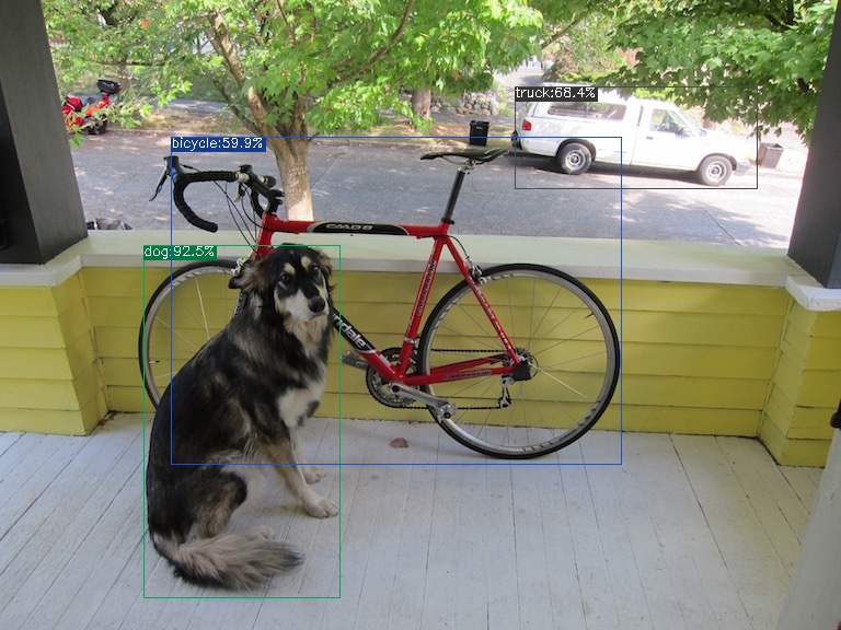
dog_f16.jpg:

alt text

dog_f32.jpg:

alt text

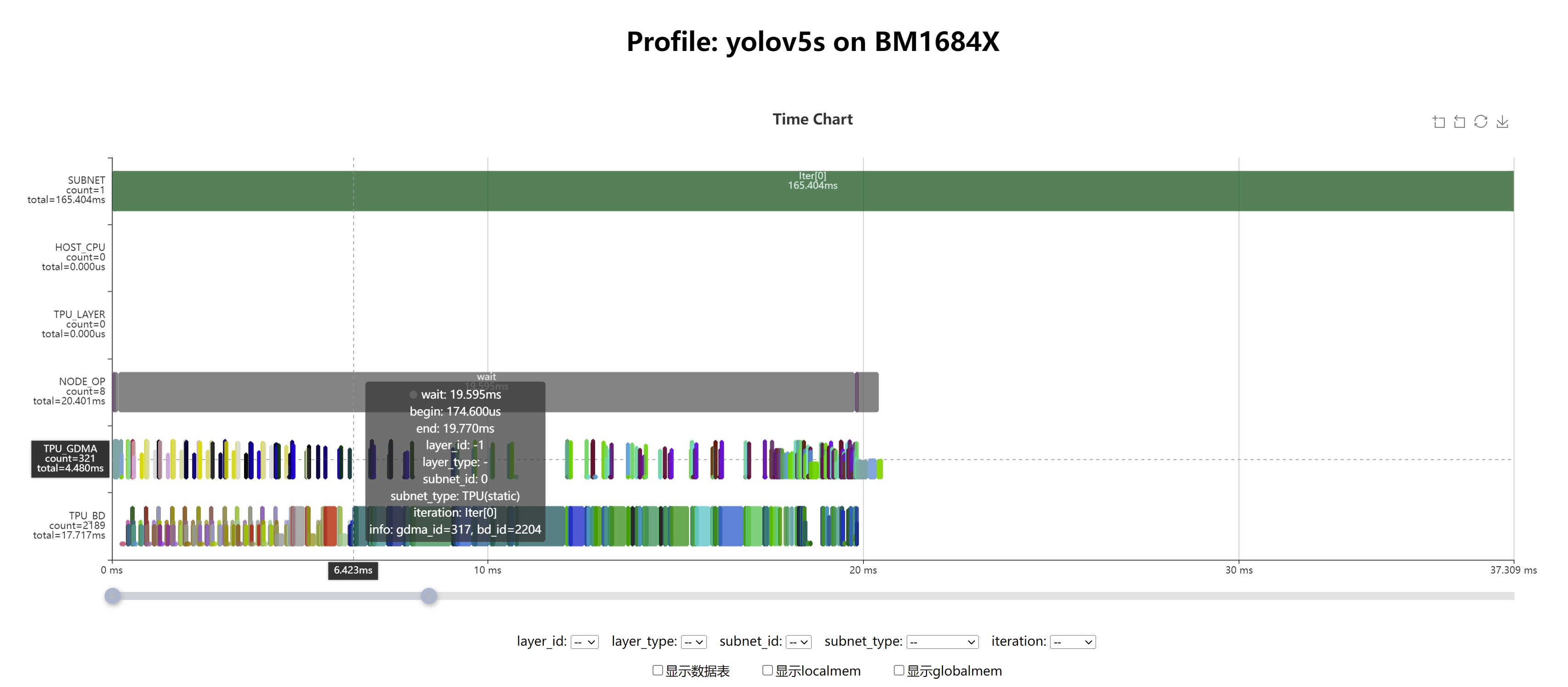
性能分析

通过利用Profile数据和TPU Profile工具，可以可视化模型的完整运行流程，从而便于进行性能分析。首先，将生成的yolov5s_bm1684x_f16.bmodel文件复制到已安装libsophon的运行环境中。与编译过程类似，运行时的Profile功能默认是关闭的，以避免在保存和传输Profile时造成额外的时间消耗。当需要启用Profile功能时，只需在运行编译好的bmodel之前设置环境变量BMRUNTIME_ENABLE_PROFILE=1。然后，使用libsophon提供的模型测试工具bmrt_test运行bmodel，以生成Profile数据。

# 通过环境变量(BMRUNTIME_ENABLE_PROFILE)使能profile, 生成二进制数据
BMRUNTIME_ENABLE_PROFILE=1 bmrt_test --bmodel resnet50_fix8b.bmodel

结果

[BMRT][load_bmodel:1734] INFO:pre net num: 0, load net num: 1
[BMRT][load_tpu_module:1830] INFO:loading firmare in bmodel
[BMRT][preload_funcs:2149] INFO: core_id=0, multi_fullnet_func_id=148
[BMRT][preload_funcs:2152] INFO: core_id=0, dynamic_fullnet_func_id=149
[BMRT][setup_profile_context:814] WARNING:bmodel do not contain any profile info
[BMRT][show_net_info:2535] INFO: ########################
[BMRT][show_net_info:2540] INFO: NetName: yolov5s, Index=0, CoreNum=1
[BMRT][show_net_info:2543] INFO: ---- stage 0 ----
[BMRT][show_net_info:2553] INFO:   Input 0) 'images' shape=[ 1 3 640 640 ] dtype=FLOAT32 scale=1 zero_point=0 device_id=0
[BMRT][show_net_info:2564] INFO:   Output 0) 'output_Concat' shape=[ 1 25200 85 ] dtype=FLOAT32 scale=1 zero_point=0 device_id=0
[BMRT][show_net_info:2564] INFO:   Output 1) '350_Transpose' shape=[ 1 3 80 80 85 ] dtype=FLOAT32 scale=1 zero_point=0 device_id=0
[BMRT][show_net_info:2564] INFO:   Output 2) '498_Transpose' shape=[ 1 3 40 40 85 ] dtype=FLOAT32 scale=1 zero_point=0 device_id=0
[BMRT][show_net_info:2564] INFO:   Output 3) '646_Transpose' shape=[ 1 3 20 20 85 ] dtype=FLOAT32 scale=1 zero_point=0 device_id=0
[BMRT][show_net_info:2567] INFO: ########################
[BMRT][bmrt_test:889] INFO:==> running network #0, name: yolov5s, loop: 0
[BMRT][bmrt_test:944] INFO:reading input #0, bytesize=4915200
[BMRT][print_array:756] INFO:  --> input_data: < 0 0 0 0 0 0 0 0 0 0 0 0 0 0 0 0 ... > len=1228800
[BMRT][write_block:324] INFO: write_block: type=1, len=36
[BMRT][write_block:324] INFO: write_block: type=8, len=44
[BMRT][end:76] INFO:bdc record_num=2189, max_record_num=1048576
[BMRT][write_block:324] INFO: write_block: type=3, len=70048
[BMRT][end:89] INFO:gdma record_num=321, max_record_num=1048576
[BMRT][write_block:324] INFO: write_block: type=4, len=61632
[BMRT][write_block:324] INFO: write_block: type=5, len=288
[BMRT][write_block:324] INFO: write_block: type=6, len=1340
[BMRT][print_note:100] INFO:*****************************************************************
[BMRT][print_note:101] INFO:* PROFILE MODE due to BMRUNTIME_ENABLE_PROFILE=1
[BMRT][print_note:102] INFO:* Note: BMRuntime will collect time data during running         *
[BMRT][print_note:103] INFO:*       that will cost extra time.                              *
[BMRT][print_note:104] INFO:* Close PROFILE Mode by "unset BMRUNTIME_ENABLE_PROFILE"
[BMRT][print_note:105] INFO:*****************************************************************
[BMRT][bmrt_test:1089] INFO:reading output #0, bytesize=8568000
[BMRT][print_array:756] INFO:  --> output ref_data: < 0 0 0 0 0 0 0 0 0 0 0 0 0 0 0 0 ... > len=2142000
[BMRT][bmrt_test:1089] INFO:reading output #1, bytesize=6528000
[BMRT][print_array:756] INFO:  --> output ref_data: < 0 0 0 0 0 0 0 0 0 0 0 0 0 0 0 0 ... > len=1632000
[BMRT][bmrt_test:1089] INFO:reading output #2, bytesize=1632000
[BMRT][print_array:756] INFO:  --> output ref_data: < 0 0 0 0 0 0 0 0 0 0 0 0 0 0 0 0 ... > len=408000
[BMRT][bmrt_test:1089] INFO:reading output #3, bytesize=408000
[BMRT][print_array:756] INFO:  --> output ref_data: < 0 0 0 0 0 0 0 0 0 0 0 0 0 0 0 0 ... > len=102000
[BMRT][bmrt_test:1139] INFO:net[yolov5s] stage[0], launch total time is 271429 us (npu 20523 us, cpu 250906 us), (launch func time 271425 us, sync 4 us)
[BMRT][bmrt_test:1146] INFO:+++ The network[yolov5s] stage[0] output_data +++
[BMRT][print_array:756] INFO:output data #0 shape: [1 25200 85 ] < 5.22443 2.85089 10.7558 10.5032 6.54244e-06 0.176123 0.00520219 0.044946 0.0045222 0.00351634 0.00180591 0.0015516 0.00476113 0.00907193 0.0473877 0.00191117 ... > len=2142000
[BMRT][print_array:756] INFO:output data #1 shape: [1 3 80 80 85 ] < 0.308533 -0.289279 0.0742412 -0.202984 -11.9372 -1.54284 -5.25346 -3.05631 -5.39422 -5.64681 -6.31488 -6.46692 -5.3425 -4.69346 -3.00084 -6.25813 ... > len=1632000
[BMRT][print_array:756] INFO:output data #2 shape: [1 3 40 40 85 ] < -0.0399987 0.252585 -0.383008 -0.521117 -11.0394 -1.3127 -5.11408 -3.31933 -5.46268 -5.97731 -5.76262 -6.10796 -5.14695 -5.37918 -2.57402 -6.29721 ... > len=408000
[BMRT][print_array:756] INFO:output data #3 shape: [1 3 20 20 85 ] < 0.714055 0.655423 -0.535399 -0.240734 -9.81843 -1.2305 -5.77227 -3.35369 -5.92415 -5.12047 -5.79011 -5.18393 -5.22128 -5.52896 -4.52387 -6.63506 ... > len=102000
[BMRT][bmrt_test:1208] INFO:load input time(s): 0.003325
[BMRT][bmrt_test:1209] INFO:pre alloc  time(s): 0.000004
[BMRT][bmrt_test:1210] INFO:calculate  time(s): 0.271429
[BMRT][bmrt_test:1211] INFO:get output time(s): 0.004142
[BMRT][bmrt_test:1212] INFO:compare    time(s): 0.001548

结果可视化

将上述步骤生成的bmprofile_data-1目录复制回Docker中的tpu-mlir工程环境。tpu-mlir提供了tpu_profile脚本，用于将生成的二进制Profile数据转换为网页文件并进行可视化。在Docker内执行以下命令：

tpu_profile bmprofile_data-1 bmprofile_out
ls bmprofile_out
# echarts.min.js  profile_data.js  result.html

执行命令后会生成bmprofile_out文件夹，在浏览器中打开bmprofile_out/result.html，即可查看Profile的图表。 alt text

AI技术栈解析及应用- 作者：张真瑜 | 山东大学智能创新研究院