引言
人工智能(AI)技术在过去十年中经历了前所未有的发展,从学术研究走向广泛的商业应用。这一快速发展不仅带来了令人瞩目的技术突破,也催生了复杂多样的软硬件生态系统。在这个快速演进的领域中,理解和掌握AI技术栈的结构和特点变得越来越重要。
本文旨在提供一个系统化的视角来审视当前AI技术栈的构成。我们将深入探讨从底层硬件到高层应用框架的各个层次,分析它们之间的相互关系,以及如何协同工作以支持现代AI系统的开发和部署。通过这种分层的方法,我们不仅可以更好地理解现有技术,还能洞察未来的发展趋势。
在接下来的章节中,我们将首先概述AI技术栈的整体架构,然后逐一深入探讨各大主流平台(如NVIDIA、AMD、Intel等)的技术特点。我们将分析每个平台在各个层次的实现,比较它们的优势和局限性,并探讨如何在实际应用中做出最优的技术选择。
通过本文,我们希望为AI研究者、开发者和决策者提供一个全面的参考框架,帮助他们在这个快速发展的领域中做出明智的技术决策,并为未来的创新铺平道路。
技术栈架构概述
在本节中,AI技术栈层次提出了一种新的分层方法,将AI技术栈分为系统软件层、运行时环境层、编程模型和语言层、计算库层以及框架模型层。这种结构不仅有助于理清各种技术之间的关系,还为开发者和研究者提供了一个系统化的视角。
其次,AI技术栈的意义探讨了这种分层方法所带来的多重优势,如实现系统化理解、促进模块化设计、精确定位性能瓶颈以及推动技术标准化等。这使得不同层次的技术能够更有效地比较与优化,为选择适合的技术方案提供了坚实依据。
最后,AI技术栈分层方法与应用详细阐述了每一层的具体执行和应用实例,包括对API调用和硬件接口的分析、编程语言的特性比较以及计算库和框架性能的评估。通过这种全面的分层分析,我们不仅能够更好地理解当前AI系统的性能特征,还为未来的技术发展与优化提供了清晰的路径。
AI 技术栈层次
人工智能技术的快速发展带来了复杂多样的软硬件生态系统。为了更好地理解和利用这些技术,我们提出了一种新的分层方法来分析AI技术栈。这种分层不仅有助于我们理清各种技术之间的关系,还为开发者、研究者和决策者提供了一个系统化的视角来审视整个AI生态系统。
AI 技术栈通常包含以下层次:
- 系统软件层:设备驱动程序、底层 API
- 运行时环境层:执行环境和运行时库
- 编程模型和语言层:特定于硬件的编程语言和模型
- 计算库层:优化的数学和深度学习库
- 框架模型层:高级深度学习框架
系统软件层是整个技术栈的基础,它直接与硬件交互,提供底层的驱动程序和API。这一层的设计和优化直接影响了整个系统的性能和稳定性。运行时环境层则在系统软件之上提供了一个抽象层,使得上层应用能够更加高效地利用硬件资源。
编程模型和语言层是开发者与系统交互的主要接口。不同的编程模型和语言反映了不同的计算范式和抽象级别,从而影响了开发效率和代码可移植性。计算库层提供了高度优化的数学和机器学习算法实现,是提升性能的关键所在。最上层的框架模型层则为开发者提供了高级的API和工具,大大简化了AI模型的开发和部署过程。
AI技术栈的的意义
AI技术栈的分层方法不仅仅是一种理论构造,它在实际应用和研究中具有深远的意义和多方面的优势:
-
系统化理解:分层结构提供了一个系统化的框架,使得复杂的AI生态系统变得更加清晰可理解。这种结构化的视角有助于开发者、研究者和决策者更好地把握整个技术领域的全貌。
-
模块化设计:分层架构促进了模块化设计的思想。每一层都有明确定义的接口和功能,这使得开发者可以专注于特定层次的优化,而不必过多考虑其他层次的复杂性。
-
技术对比:通过分层,我们可以在相同的层次上比较不同平台或技术的实现。这种横向对比有助于识别各种技术的优势和劣势,为技术选型提供客观依据。
-
性能优化:分层结构使得性能瓶颈的定位变得更加精确。开发者可以针对特定层次进行优化,而不是盲目地对整个系统进行调整。
-
跨层优化:虽然分层提供了清晰的结构,但它也为跨层优化提供了可能。了解各层之间的相互作用,可以实现更深层次的系统优化。
-
标准化促进:分层架构为制定行业标准提供了基础。不同层次的标准化有助于提高技术的互操作性和可移植性。
总的来说AI技术栈提供了一个清晰的结构来理解和比较不同的AI技术。例如,当我们比较NVIDIA的CUDA和AMD的ROCm时,我们可以在每一层级进行对比,从而全面地评估两种技术的异同。这不仅有助于技术选型,还为性能优化提供了指导。
从开发者的角度来看,这种分层结构使得他们可以根据自己的需求和专长选择合适的切入点。例如,深度学习研究者可能主要关注框架模型层,而系统优化专家则可能更多地工作在底层。同时,这种分层也有利于跨层优化,开发者可以根据需要在不同层次间进行调优。
从行业发展的角度来看,这种分层结构也反映了AI技术的发展趋势。我们看到,在每一层都有不断涌现的新技术,如编程模型层的SYCL,计算库层的oneDNN,以及框架模型层的各种新兴深度学习框架。这种分层结构有助于我们更好地理解这些新技术在整个生态系统中的位置和作用。
通过这种分层方法,我们不仅能更好地理解和利用现有技术,还能为未来的技术发展提供清晰的路径和方向。
AI技术栈分层方法与应用
AI 技术栈的每个层次分析都有其特定方法和应用demo。本节将阐述后续章节的分析逻辑,解释为什么要进行这样的分层分析,以及每层分析的意义和应用。通过深入理解每个层次的特点,我们可以更好地利用 AI 技术栈来开发和优化 AI 系统。
2.3.1 系统软件层和运行时环境层
在后续章节中,这一层的分析主要聚焦于 API 调用和硬件接口,目的是理解不同技术路线在相同硬件平台下如何与底层系统交互。
-
API 调用分析
- 目的:了解各种 AI 框架和库如何与底层硬件交互
- 意义:揭示谁实际使用了 CUDA Driver API,CUDA Runtime API等底层接口,有助于理解不同技术路线调用相同接口的异同。
-
硬件接口比较
- 目的:比较不同 AI 技术栈在访问相同硬件时的方式
- 意义:了解不同方案的底层实现差异,为性能优化提供思路
-
扩展性分析
- 目的:研究如何为新硬件或新接口扩展现有系统
- 意义:为未来硬件适配和系统升级提供指导
这一层不进行直接的性能比较,因为系统软件层的差异通常不是性能瓶颈的主要来源。相反,我们关注的是不同方案如何利用底层资源,这为理解整体性能提供了基础。
2.3.2 编程模型和语言层
这一层的分析主要起到教学和概念引入的作用,为后续的深入分析奠定基础。
-
语言特性对比
- 目的:展示不同编程语言(如 Python、C++、CUDA)在 AI 开发中的应用
- 意义:帮助理解语言选择对开发效率和性能的影响
-
算子编写示例
- 目的:提供常见 AI 算子(如卷积、矩阵乘法)的实现示例
- 意义:深入理解算子工作原理,为后续优化提供思路
-
并行计算模型介绍
- 目的:解释 CUDA、OpenCL 等并行计算模型的基本概念
- 意义:为理解 GPU 加速原理和优化方法打下基础
这一层的分析不直接进行性能比较,而是为读者提供必要的背景知识,使他们能够理解后续章节中更复杂的性能分析和优化策略。
2.3.3 计算库层、框架模型层
在这些高层次中,我们将基于现有的 AI Benchmark进行更深入的应用和研究。
-
计算库性能分析
- 目的:比较不同计算库(如 cuDNN、oneDNN)在常见算子上的性能
- 意义:了解底层库对整体性能的影响,指导算子优化和选择
-
框架性能对比
- 目的:评估不同深度学习框架(如 TensorFlow、PyTorch)在相同任务上的性能
- 意义:帮助开发者选择适合特定任务的框架,了解框架优化的重要性
-
模型层 Benchmark 扩展
- 目的:将更多类型的模型纳入 AI Benchmark
- 意义:提供更全面的性能评估,覆盖更广泛的应用场景
-
算子级 Benchmark
- 目的:开发针对单个算子的性能测试套件
- 意义:深入了解性能瓶颈,指导底层优化
-
安装和部署指南
- 目的:基于 Benchmark 结果,提供模型选择和部署的最佳实践
- 意义:帮助用户根据自身硬件和需求选择最合适的模型和框架
这些高层次的分析直接关系到 AI 系统的最终性能。通过全面的 Benchmark 和分析,我们可以获得不同组件和配置的详细性能数据,从而指导实际应用中的选择和优化。
通过这种分层分析方法,我们可以全面地理解 AI 技术栈的各个层次,从底层硬件接口到高层模型性能。这种方法不仅有助于理解当前 AI 系统的性能特征,还为未来的优化和创新提供了清晰的路径。在后续章节中,我们将基于这个框架,提供具体的示例和深入分析,展示如何在实际应用中利用这种分层思想来优化 AI 系统性能。
NVIDIA 平台
NVIDIA 是一家领先的图形处理器(GPU)制造商,在人工智能(AI)领域拥有广泛的技术布局。NVIDIA 的 GPU 在深度学习、机器学习等 AI 应用中发挥着关键作用,为开发者提供了强大的硬件加速能力。
除了硬件,NVIDIA 平台还具备了一系列软件工具和框架,帮助开发者更好地利用 GPU 进行 AI 开发。接下来我们将介绍以下几个重要的 NVIDIA 平台相关技术并在后续通过AI技术栈进行深入分析:
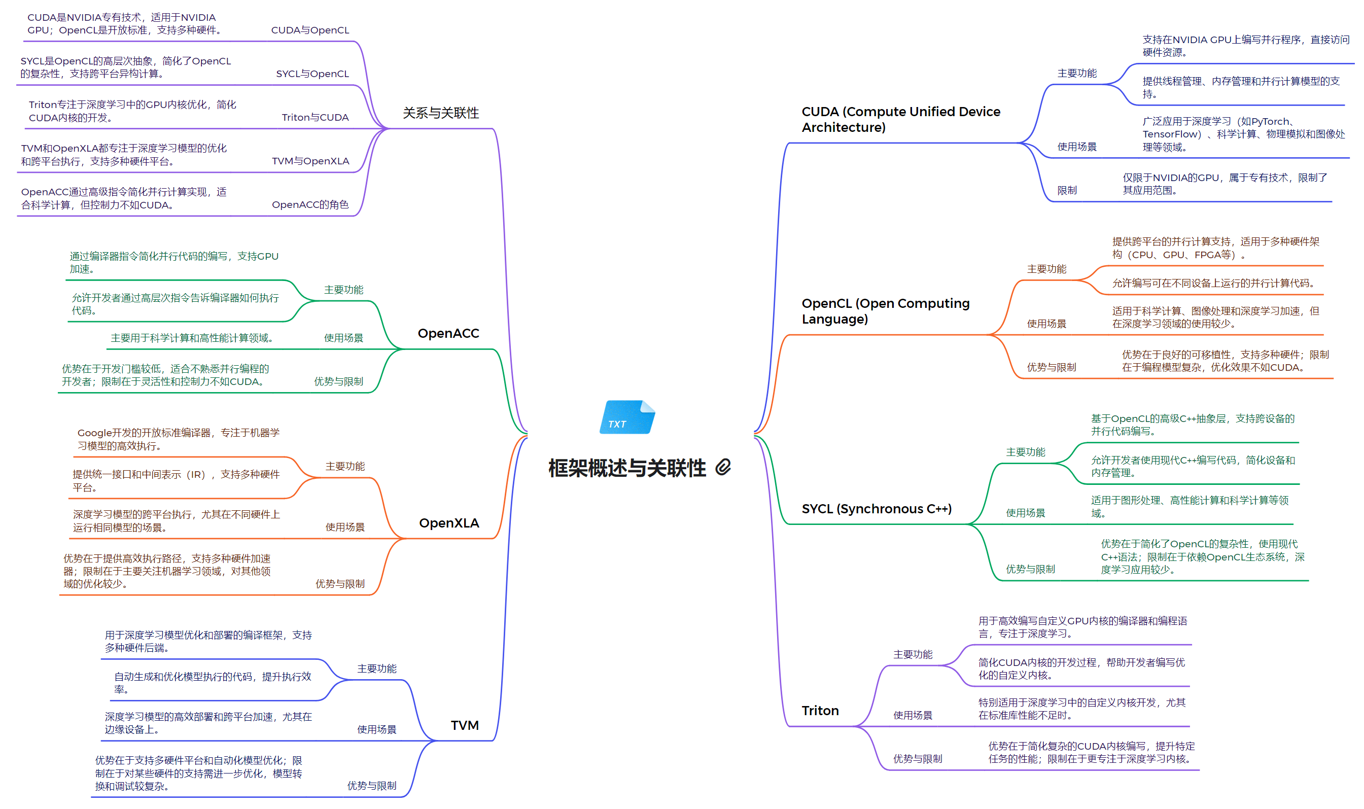
CUDA
CUDA 是 NVIDIA 开发的一种通用并行计算架构,可以利用 NVIDIA GPU 进行高性能计算。CUDA 提供了一个编程模型和指令集,使开发者能够编写高效的并行程序,充分发挥 GPU 的计算能力。
OpenCL
OpenCL 是一种开放标准的并行计算框架,可以在异构计算平台(如 CPU、GPU、FPGA 等)上运行。与 CUDA 类似,OpenCL 也为开发者提供了编程模型和指令集,用于开发并行应用程序。
SYCL (DPC++)
SYCL 是基于 OpenCL 的一种C++层次化的异构编程模型。DPC++ 是 SYCL 的一种实现,由 Intel 开发并贡献给 LLVM 社区。DPC++ 支持在 CPU、GPU 和其他加速器上运行并行计算任务。
Triton
Triton 是 NVIDIA 开发的一个高性能推理服务器,可以部署和运行各种深度学习模型。Triton 支持多种框架(TensorFlow、PyTorch 等)和部署环境,为开发者提供了灵活的模型部署解决方案。
Apache TVM
Apache TVM 是一个开源的端到端机器学习编译器栈,可以针对不同的硬件平台(CPU、GPU、FPGA 等)优化机器学习模型的性能。TVM 可以与 NVIDIA 的 CUDA 和 Triton 等技术集成使用。
OpenXLA
OpenXLA 是 Google 开源的一个机器学习编译器框架,可以将不同的机器学习模型编译为高效的原生代码。NVIDIA 正在与 Google 合作,将 OpenXLA 与 CUDA 等技术进行集成。
OpenACC
OpenACC 是一种指令级并行编程模型,可以让开发者更容易地将现有的 C、C++ 或 Fortran 代码移植到 GPU 上运行。OpenACC 为开发者提供了一种声明式的编程方式,无需深入了解 GPU 的底层细节。
CUDA
CUDA(Compute Unified Device Architecture)是NVIDIA公司开发的一种并行计算平台和编程模型。它允许软件开发者利用NVIDIA的GPU(图形处理单元)进行通用计算,大大提高了计算密集型任务的处理速度。
CUDA的核心概念
-
异构计算:CUDA基于CPU和GPU协同工作的异构计算模型。CPU负责管理程序流程和数据传输,而GPU负责并行计算任务。
-
线程层次结构:CUDA采用了独特的线程层次结构:
- 线程(Thread):最基本的执行单元
- 线程块(Block):由多个线程组成
- 网格(Grid):由多个线程块组成
-
内存层次结构:CUDA定义了多层内存结构,包括全局内存、共享内存、本地内存和寄存器等,以优化数据访问和管理。
CUDA的主要特点
-
高性能并行计算:利用GPU的大量计算核心,CUDA可以实现高度并行的计算,显著提升性能。
-
灵活的编程模型:CUDA扩展了C/C++语言,使开发者能够方便地编写并行程序。
-
丰富的库和工具:NVIDIA提供了众多优化库(如cuBLAS、cuDNN等)和开发工具(如CUDA Toolkit、NSight等)。
-
跨平台支持:CUDA支持Windows、Linux和macOS等多种操作系统。
-
自动伸缩性:CUDA程序可以自动适应不同的GPU硬件,实现代码的可移植性。
编写CUDA程序的基本步骤
- 初始化数据
- 将数据从主机内存传输到GPU内存
- 调用CUDA核函数执行并行计算
- 将结果从GPU内存传回主机内存
- 释放分配的内存资源
CUDA作为一种强大的并行计算平台,为开发者提供了充分利用GPU计算能力的工具。它在科学计算、人工智能等领域发挥着重要作用,推动了高性能计算的发展。然而,有效利用CUDA需要对并行编程和GPU架构有深入的理解,这也是许多开发者面临的挑战。
技术栈架构
1. 系统软件层
- NVIDIA GPU 驱动:为 GPU 提供基本的系统级支持
- CUDA Driver API:低级 API,提供对 GPU 的直接控制
- 允许直接管理设备、内存分配和程序执行
- 适用于需要细粒度控制的高级应用
- 提供与 NVIDIA GPU 硬件交互的底层接口
2. 运行时环境层
- CUDA Runtime API:高级 API,简化了 GPU 编程,自动管理许多底层细节
- 提供更高级的抽象,简化了 GPU 的使用
- 自动处理上下文管理和程序加载等任务
- 更适合一般开发者使用,提供了更好的易用性
3. 编程模型和语言层
- CUDA C/C++:扩展了 C/C++ 语言,允许开发者编写在 GPU 上运行的并行程序
- 允许在 CPU 和 GPU 上混合编程
- 使用 CUDA 特定语法(如
__global__)来定义 GPU 函数 - 通过
<<<>>>语法启动内核 - 支持主机代码和设备代码的混合编写
4. 计算库层
- cuBLAS:用于线性代数计算的库
- 提供 GPU 加速的矩阵运算和 BLAS 功能
- 广泛用于深度学习中的矩阵计算
- NCCL:用于多 GPU 通信的库
- 支持多 GPU 之间的高效通信和数据交换
- 主要用于分布式深度学习训练
- 其他专用算子库(如 cuDNN)
5. 框架模型层
- PyTorch:支持动态计算图的深度学习框架
- 通过
torch.cuda模块提供 CUDA 功能 - 自动管理 GPU 内存
- 支持 CPU 和 GPU 之间的数据转移
- 通过
- TensorFlow:支持静态和动态计算图的深度学习框架
- 通过 XLA 编译器优化 GPU 代码执行
- 提供高级 API,简化了 CUDA API 的使用
关系解析
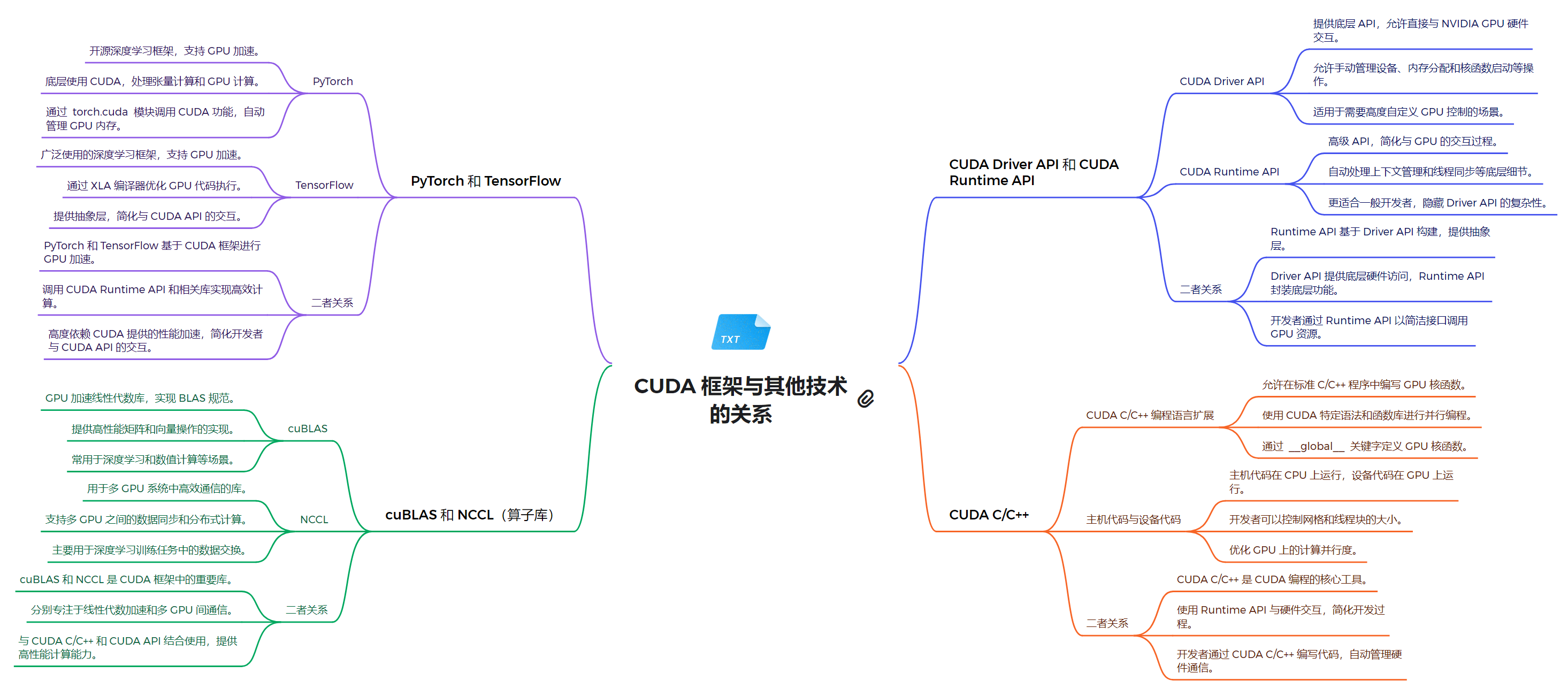
- CUDA Driver API 和 CUDA Runtime API 的关系
- Runtime API 构建在 Driver API 之上,提供了更高级的抽象
- Driver API 提供更多控制,但使用更复杂
- Runtime API 更容易上手,隐藏了 Driver API 的复杂性
- 开发者可以根据需求选择使用 Runtime API 或直接使用 Driver API
- PyTorch 和 TensorFlow 与 CUDA 的关系
- 两者都基于 CUDA Runtime API 实现 GPU 加速
- 提供了高级抽象,使开发者无需直接编写 CUDA 代码
- 支持自动微分和 GPU 加速的深度学习模型训练
- PyTorch 和 TensorFlow 都支持 CPU 和 GPU 训练
- cuBLAS 和 NCCL 与 CUDA 的关系
- 这些库是 CUDA 生态系统的重要组成部分
- 它们利用 CUDA 的并行计算能力,提供高性能的数学运算和通信功能
- 与 CUDA C/C++ 和 CUDA API 结合使用,提供高性能计算能力
通过以上结构,CUDA 技术路线为开发者提供了从底层硬件控制到高层应用开发的全面支持,使得 GPU 并行计算的强大功能能够被有效地应用到各种计算密集型任务中。
系统软件层
编写了一个使用 CUDA Driver API 的程序,列出系统中可用的 CUDA 设备,获取设备的名称、计算能力、驱动版本和全局内存大小,并创建和销毁 CUDA 上下文。
-
初始化 CUDA 驱动
-
获取可用 CUDA 设备的数量,并循环遍历每个设备
-
使用 cuDeviceGetName、cuDeviceGetAttribute 、cuDeviceTotalMem和cuDriverGetVersion 获取设备的详细信息
-
创建 CUDA 上下文并设置为当前上下文
-
输出设备信息,并在结束时销毁上下文
示例代码:
#include <iostream>
#include <cuda.h>

// Check the return value of CUDA functions and print error message on failure
void checkCudaErrors(CUresult result) {
    if (result != CUDA_SUCCESS) {
        const char *errorStr;
        cuGetErrorString(result, &errorStr);
        std::cerr << "CUDA Error: " << errorStr << std::endl;
        exit(EXIT_FAILURE);
    }
}

// Print information about a CUDA device
void printDeviceInfo(CUdevice device) {
    int driverVersion = 0;
    char deviceName[256];
    // Get device name
    checkCudaErrors(cuDeviceGetName(deviceName, sizeof(deviceName), device));

    int computeCapabilityMajor, computeCapabilityMinor;
    // Get the major and minor version of compute capability
    checkCudaErrors(cuDeviceGetAttribute(&computeCapabilityMajor, CU_DEVICE_ATTRIBUTE_COMPUTE_CAPABILITY_MAJOR, device));
    checkCudaErrors(cuDeviceGetAttribute(&computeCapabilityMinor, CU_DEVICE_ATTRIBUTE_COMPUTE_CAPABILITY_MINOR, device));

    size_t totalGlobalMem;
    checkCudaErrors(cuDeviceTotalMem(&totalGlobalMem, device));
    checkCudaErrors(cuDriverGetVersion(&driverVersion));

    // Print device details
    std::cout << "Device Name: " << deviceName << std::endl;
    std::cout << "Compute Capability: " << computeCapabilityMajor << "." << computeCapabilityMinor << std::endl;
    std::cout << "CUDA Driver Version: " << driverVersion / 1000 << "." << (driverVersion % 100) / 10 << std::endl;
    std::cout << "Total Global Memory: " << totalGlobalMem / (1024 * 1024) << " MB" << std::endl;
}

int main() {
    // Initialize CUDA
    checkCudaErrors(cuInit(0));

    // Get the number of available CUDA devices
    int deviceCount;
    checkCudaErrors(cuDeviceGetCount(&deviceCount));
    std::cout << "Number of CUDA Devices: " << deviceCount << std::endl;

    CUdevice device;
    // Iterate through each device and print its information
    for (int i = 0; i < deviceCount; i++) {
        checkCudaErrors(cuDeviceGet(&device, i));
        printDeviceInfo(device);
        std::cout << std::endl;
    }

    CUcontext context;
    // Create a CUDA context and set it as the current context
    checkCudaErrors(cuCtxCreate(&context, 0, deviceCount > 0 ? device : 0));
    checkCudaErrors(cuCtxSetCurrent(context));

    std::cout << "CUDA context created successfully." << std::endl;

    checkCudaErrors(cuCtxDestroy(context));

    return 0;
}
结果:
Number of CUDA Devices: 1
Device Name: NVIDIA GeForce RTX 4080 SUPER
Compute Capability: 8.9
CUDA Driver Version: 12.4
Total Global Memory: 16072 MB

CUDA context created successfully.
运行时环境层
CUDA Runtime API 是 NVIDIA 提供的用于管理和使用 GPU 资源的接口,旨在简化开发者与 CUDA 设备之间的交互。该 API 支持多种功能,包括设备查询、内存管理和流控制等,极大地提高了 GPU 编程的效率和可用性。
参考仓库地址:deviceQuery
示例代码如下:
/* Copyright (c) 2022, NVIDIA CORPORATION. All rights reserved.
 *
 * Redistribution and use in source and binary forms, with or without
 * modification, are permitted provided that the following conditions
 * are met:
 *  * Redistributions of source code must retain the above copyright
 *    notice, this list of conditions and the following disclaimer.
 *  * Redistributions in binary form must reproduce the above copyright
 *    notice, this list of conditions and the following disclaimer in the
 *    documentation and/or other materials provided with the distribution.
 *  * Neither the name of NVIDIA CORPORATION nor the names of its
 *    contributors may be used to endorse or promote products derived
 *    from this software without specific prior written permission.
 *
 * THIS SOFTWARE IS PROVIDED BY THE COPYRIGHT HOLDERS ``AS IS'' AND ANY
 * EXPRESS OR IMPLIED WARRANTIES, INCLUDING, BUT NOT LIMITED TO, THE
 * IMPLIED WARRANTIES OF MERCHANTABILITY AND FITNESS FOR A PARTICULAR
 * PURPOSE ARE DISCLAIMED.  IN NO EVENT SHALL THE COPYRIGHT OWNER OR
 * CONTRIBUTORS BE LIABLE FOR ANY DIRECT, INDIRECT, INCIDENTAL, SPECIAL,
 * EXEMPLARY, OR CONSEQUENTIAL DAMAGES (INCLUDING, BUT NOT LIMITED TO,
 * PROCUREMENT OF SUBSTITUTE GOODS OR SERVICES; LOSS OF USE, DATA, OR
 * PROFITS; OR BUSINESS INTERRUPTION) HOWEVER CAUSED AND ON ANY THEORY
 * OF LIABILITY, WHETHER IN CONTRACT, STRICT LIABILITY, OR TORT
 * (INCLUDING NEGLIGENCE OR OTHERWISE) ARISING IN ANY WAY OUT OF THE USE
 * OF THIS SOFTWARE, EVEN IF ADVISED OF THE POSSIBILITY OF SUCH DAMAGE.
 */

/* This sample queries the properties of the CUDA devices present in the system
 * via CUDA Runtime API. */

// std::system includes

#include <cuda_runtime.h>
#include <helper_cuda.h>

#include <iostream>
#include <memory>
#include <string>

int *pArgc = NULL;
char **pArgv = NULL;

#if CUDART_VERSION < 5000

// This function wraps the CUDA Driver API into a template function
template <class T>
inline void getCudaAttribute(T *attribute, CUdevice_attribute device_attribute,
                             int device) {
  CUresult error = cuDeviceGetAttribute(attribute, device_attribute, device);

  if (CUDA_SUCCESS != error) {
    fprintf(
        stderr,
        "cuSafeCallNoSync() Driver API error = %04d from file <%s>, line %i.\n",
        error, __FILE__, __LINE__);

    exit(EXIT_FAILURE);
  }
}

#endif /* CUDART_VERSION < 5000 */

////////////////////////////////////////////////////////////////////////////////
// Program main
////////////////////////////////////////////////////////////////////////////////
int main(int argc, char **argv) {
  pArgc = &argc;
  pArgv = argv;

  printf("%s Starting...\n\n", argv[0]);
  printf(
      " CUDA Device Query (Runtime API) version (CUDART static linking)\n\n");

  int deviceCount = 0;
  cudaError_t error_id = cudaGetDeviceCount(&deviceCount);

  if (error_id != cudaSuccess) {
    printf("cudaGetDeviceCount returned %d\n-> %s\n",
           static_cast<int>(error_id), cudaGetErrorString(error_id));
    printf("Result = FAIL\n");
    exit(EXIT_FAILURE);
  }

  // This function call returns 0 if there are no CUDA capable devices.
  if (deviceCount == 0) {
    printf("There are no available device(s) that support CUDA\n");
  } else {
    printf("Detected %d CUDA Capable device(s)\n", deviceCount);
  }

  int dev, driverVersion = 0, runtimeVersion = 0;

  for (dev = 0; dev < deviceCount; ++dev) {
    cudaSetDevice(dev);
    cudaDeviceProp deviceProp;
    cudaGetDeviceProperties(&deviceProp, dev);

    printf("\nDevice %d: \"%s\"\n", dev, deviceProp.name);

    // Console log
    cudaDriverGetVersion(&driverVersion);
    cudaRuntimeGetVersion(&runtimeVersion);
    printf("  CUDA Driver Version / Runtime Version          %d.%d / %d.%d\n",
           driverVersion / 1000, (driverVersion % 100) / 10,
           runtimeVersion / 1000, (runtimeVersion % 100) / 10);
    printf("  CUDA Capability Major/Minor version number:    %d.%d\n",
           deviceProp.major, deviceProp.minor);

    char msg[256];
#if defined(WIN32) || defined(_WIN32) || defined(WIN64) || defined(_WIN64)
    sprintf_s(msg, sizeof(msg),
              "  Total amount of global memory:                 %.0f MBytes "
              "(%llu bytes)\n",
              static_cast<float>(deviceProp.totalGlobalMem / 1048576.0f),
              (unsigned long long)deviceProp.totalGlobalMem);
#else
    snprintf(msg, sizeof(msg),
             "  Total amount of global memory:                 %.0f MBytes "
             "(%llu bytes)\n",
             static_cast<float>(deviceProp.totalGlobalMem / 1048576.0f),
             (unsigned long long)deviceProp.totalGlobalMem);
#endif
    printf("%s", msg);

    printf("  (%03d) Multiprocessors, (%03d) CUDA Cores/MP:    %d CUDA Cores\n",
           deviceProp.multiProcessorCount,
           _ConvertSMVer2Cores(deviceProp.major, deviceProp.minor),
           _ConvertSMVer2Cores(deviceProp.major, deviceProp.minor) *
               deviceProp.multiProcessorCount);
    printf(
        "  GPU Max Clock rate:                            %.0f MHz (%0.2f "
        "GHz)\n",
        deviceProp.clockRate * 1e-3f, deviceProp.clockRate * 1e-6f);

#if CUDART_VERSION >= 5000
    // This is supported in CUDA 5.0 (runtime API device properties)
    printf("  Memory Clock rate:                             %.0f Mhz\n",
           deviceProp.memoryClockRate * 1e-3f);
    printf("  Memory Bus Width:                              %d-bit\n",
           deviceProp.memoryBusWidth);

    if (deviceProp.l2CacheSize) {
      printf("  L2 Cache Size:                                 %d bytes\n",
             deviceProp.l2CacheSize);
    }

#else
    // This only available in CUDA 4.0-4.2 (but these were only exposed in the
    // CUDA Driver API)
    int memoryClock;
    getCudaAttribute<int>(&memoryClock, CU_DEVICE_ATTRIBUTE_MEMORY_CLOCK_RATE,
                          dev);
    printf("  Memory Clock rate:                             %.0f Mhz\n",
           memoryClock * 1e-3f);
    int memBusWidth;
    getCudaAttribute<int>(&memBusWidth,
                          CU_DEVICE_ATTRIBUTE_GLOBAL_MEMORY_BUS_WIDTH, dev);
    printf("  Memory Bus Width:                              %d-bit\n",
           memBusWidth);
    int L2CacheSize;
    getCudaAttribute<int>(&L2CacheSize, CU_DEVICE_ATTRIBUTE_L2_CACHE_SIZE, dev);

    if (L2CacheSize) {
      printf("  L2 Cache Size:                                 %d bytes\n",
             L2CacheSize);
    }

#endif

    printf(
        "  Maximum Texture Dimension Size (x,y,z)         1D=(%d), 2D=(%d, "
        "%d), 3D=(%d, %d, %d)\n",
        deviceProp.maxTexture1D, deviceProp.maxTexture2D[0],
        deviceProp.maxTexture2D[1], deviceProp.maxTexture3D[0],
        deviceProp.maxTexture3D[1], deviceProp.maxTexture3D[2]);
    printf(
        "  Maximum Layered 1D Texture Size, (num) layers  1D=(%d), %d layers\n",
        deviceProp.maxTexture1DLayered[0], deviceProp.maxTexture1DLayered[1]);
    printf(
        "  Maximum Layered 2D Texture Size, (num) layers  2D=(%d, %d), %d "
        "layers\n",
        deviceProp.maxTexture2DLayered[0], deviceProp.maxTexture2DLayered[1],
        deviceProp.maxTexture2DLayered[2]);

    printf("  Total amount of constant memory:               %zu bytes\n",
           deviceProp.totalConstMem);
    printf("  Total amount of shared memory per block:       %zu bytes\n",
           deviceProp.sharedMemPerBlock);
    printf("  Total shared memory per multiprocessor:        %zu bytes\n",
           deviceProp.sharedMemPerMultiprocessor);
    printf("  Total number of registers available per block: %d\n",
           deviceProp.regsPerBlock);
    printf("  Warp size:                                     %d\n",
           deviceProp.warpSize);
    printf("  Maximum number of threads per multiprocessor:  %d\n",
           deviceProp.maxThreadsPerMultiProcessor);
    printf("  Maximum number of threads per block:           %d\n",
           deviceProp.maxThreadsPerBlock);
    printf("  Max dimension size of a thread block (x,y,z): (%d, %d, %d)\n",
           deviceProp.maxThreadsDim[0], deviceProp.maxThreadsDim[1],
           deviceProp.maxThreadsDim[2]);
    printf("  Max dimension size of a grid size    (x,y,z): (%d, %d, %d)\n",
           deviceProp.maxGridSize[0], deviceProp.maxGridSize[1],
           deviceProp.maxGridSize[2]);
    printf("  Maximum memory pitch:                          %zu bytes\n",
           deviceProp.memPitch);
    printf("  Texture alignment:                             %zu bytes\n",
           deviceProp.textureAlignment);
    printf(
        "  Concurrent copy and kernel execution:          %s with %d copy "
        "engine(s)\n",
        (deviceProp.deviceOverlap ? "Yes" : "No"), deviceProp.asyncEngineCount);
    printf("  Run time limit on kernels:                     %s\n",
           deviceProp.kernelExecTimeoutEnabled ? "Yes" : "No");
    printf("  Integrated GPU sharing Host Memory:            %s\n",
           deviceProp.integrated ? "Yes" : "No");
    printf("  Support host page-locked memory mapping:       %s\n",
           deviceProp.canMapHostMemory ? "Yes" : "No");
    printf("  Alignment requirement for Surfaces:            %s\n",
           deviceProp.surfaceAlignment ? "Yes" : "No");
    printf("  Device has ECC support:                        %s\n",
           deviceProp.ECCEnabled ? "Enabled" : "Disabled");
#if defined(WIN32) || defined(_WIN32) || defined(WIN64) || defined(_WIN64)
    printf("  CUDA Device Driver Mode (TCC or WDDM):         %s\n",
           deviceProp.tccDriver ? "TCC (Tesla Compute Cluster Driver)"
                                : "WDDM (Windows Display Driver Model)");
#endif
    printf("  Device supports Unified Addressing (UVA):      %s\n",
           deviceProp.unifiedAddressing ? "Yes" : "No");
    printf("  Device supports Managed Memory:                %s\n",
           deviceProp.managedMemory ? "Yes" : "No");
    printf("  Device supports Compute Preemption:            %s\n",
           deviceProp.computePreemptionSupported ? "Yes" : "No");
    printf("  Supports Cooperative Kernel Launch:            %s\n",
           deviceProp.cooperativeLaunch ? "Yes" : "No");
    printf("  Supports MultiDevice Co-op Kernel Launch:      %s\n",
           deviceProp.cooperativeMultiDeviceLaunch ? "Yes" : "No");
    printf("  Device PCI Domain ID / Bus ID / location ID:   %d / %d / %d\n",
           deviceProp.pciDomainID, deviceProp.pciBusID, deviceProp.pciDeviceID);

    const char *sComputeMode[] = {
        "Default (multiple host threads can use ::cudaSetDevice() with device "
        "simultaneously)",
        "Exclusive (only one host thread in one process is able to use "
        "::cudaSetDevice() with this device)",
        "Prohibited (no host thread can use ::cudaSetDevice() with this "
        "device)",
        "Exclusive Process (many threads in one process is able to use "
        "::cudaSetDevice() with this device)",
        "Unknown", NULL};
    printf("  Compute Mode:\n");
    printf("     < %s >\n", sComputeMode[deviceProp.computeMode]);
  }

  // If there are 2 or more GPUs, query to determine whether RDMA is supported
  if (deviceCount >= 2) {
    cudaDeviceProp prop[64];
    int gpuid[64];  // we want to find the first two GPUs that can support P2P
    int gpu_p2p_count = 0;

    for (int i = 0; i < deviceCount; i++) {
      checkCudaErrors(cudaGetDeviceProperties(&prop[i], i));

      // Only boards based on Fermi or later can support P2P
      if ((prop[i].major >= 2)
#if defined(WIN32) || defined(_WIN32) || defined(WIN64) || defined(_WIN64)
          // on Windows (64-bit), the Tesla Compute Cluster driver for windows
          // must be enabled to support this
          && prop[i].tccDriver
#endif
          ) {
        // This is an array of P2P capable GPUs
        gpuid[gpu_p2p_count++] = i;
      }
    }

    // Show all the combinations of support P2P GPUs
    int can_access_peer;

    if (gpu_p2p_count >= 2) {
      for (int i = 0; i < gpu_p2p_count; i++) {
        for (int j = 0; j < gpu_p2p_count; j++) {
          if (gpuid[i] == gpuid[j]) {
            continue;
          }
          checkCudaErrors(
              cudaDeviceCanAccessPeer(&can_access_peer, gpuid[i], gpuid[j]));
          printf("> Peer access from %s (GPU%d) -> %s (GPU%d) : %s\n",
                 prop[gpuid[i]].name, gpuid[i], prop[gpuid[j]].name, gpuid[j],
                 can_access_peer ? "Yes" : "No");
        }
      }
    }
  }

  // csv masterlog info
  // *****************************
  // exe and CUDA driver name
  printf("\n");
  std::string sProfileString = "deviceQuery, CUDA Driver = CUDART";
  char cTemp[16];

  // driver version
  sProfileString += ", CUDA Driver Version = ";
#if defined(WIN32) || defined(_WIN32) || defined(WIN64) || defined(_WIN64)
  sprintf_s(cTemp, 10, "%d.%d", driverVersion / 1000,
            (driverVersion % 100) / 10);
#else
  snprintf(cTemp, sizeof(cTemp), "%d.%d", driverVersion / 1000,
           (driverVersion % 100) / 10);
#endif
  sProfileString += cTemp;

  // Runtime version
  sProfileString += ", CUDA Runtime Version = ";
#if defined(WIN32) || defined(_WIN32) || defined(WIN64) || defined(_WIN64)
  sprintf_s(cTemp, 10, "%d.%d", runtimeVersion / 1000,
            (runtimeVersion % 100) / 10);
#else
  snprintf(cTemp, sizeof(cTemp), "%d.%d", runtimeVersion / 1000,
           (runtimeVersion % 100) / 10);
#endif
  sProfileString += cTemp;

  // Device count
  sProfileString += ", NumDevs = ";
#if defined(WIN32) || defined(_WIN32) || defined(WIN64) || defined(_WIN64)
  sprintf_s(cTemp, 10, "%d", deviceCount);
#else
  snprintf(cTemp, sizeof(cTemp), "%d", deviceCount);
#endif
  sProfileString += cTemp;
  sProfileString += "\n";
  printf("%s", sProfileString.c_str());

  printf("Result = PASS\n");

  // finish
  exit(EXIT_SUCCESS);
}
结果:
./Samples/1_Utilities/deviceQuery/deviceQuery Starting...

 CUDA Device Query (Runtime API) version (CUDART static linking)

Detected 1 CUDA Capable device(s)

Device 0: "NVIDIA GeForce RTX 4080 SUPER"
  CUDA Driver Version / Runtime Version          12.4 / 12.3
  CUDA Capability Major/Minor version number:    8.9
  Total amount of global memory:                 16072 MBytes (16852844544 bytes)
  (080) Multiprocessors, (128) CUDA Cores/MP:    10240 CUDA Cores
  GPU Max Clock rate:                            2550 MHz (2.55 GHz)
  Memory Clock rate:                             11501 Mhz
  Memory Bus Width:                              256-bit
  L2 Cache Size:                                 67108864 bytes
  Maximum Texture Dimension Size (x,y,z)         1D=(131072), 2D=(131072, 65536), 3D=(16384, 16384, 16384)
  Maximum Layered 1D Texture Size, (num) layers  1D=(32768), 2048 layers
  Maximum Layered 2D Texture Size, (num) layers  2D=(32768, 32768), 2048 layers
  Total amount of constant memory:               65536 bytes
  Total amount of shared memory per block:       49152 bytes
  Total shared memory per multiprocessor:        102400 bytes
  Total number of registers available per block: 65536
  Warp size:                                     32
  Maximum number of threads per multiprocessor:  1536
  Maximum number of threads per block:           1024
  Max dimension size of a thread block (x,y,z): (1024, 1024, 64)
  Max dimension size of a grid size    (x,y,z): (2147483647, 65535, 65535)
  Maximum memory pitch:                          2147483647 bytes
  Texture alignment:                             512 bytes
  Concurrent copy and kernel execution:          Yes with 2 copy engine(s)
  Run time limit on kernels:                     Yes
  Integrated GPU sharing Host Memory:            No
  Support host page-locked memory mapping:       Yes
  Alignment requirement for Surfaces:            Yes
  Device has ECC support:                        Disabled
  Device supports Unified Addressing (UVA):      Yes
  Device supports Managed Memory:                Yes
  Device supports Compute Preemption:            Yes
  Supports Cooperative Kernel Launch:            Yes
  Supports MultiDevice Co-op Kernel Launch:      Yes
  Device PCI Domain ID / Bus ID / location ID:   0 / 1 / 0
  Compute Mode:
     < Default (multiple host threads can use ::cudaSetDevice() with device simultaneously) >

deviceQuery, CUDA Driver = CUDART, CUDA Driver Version = 12.4, CUDA Runtime Version = 12.3, NumDevs = 1
Result = PASS
编程模型和语言层
CUDA 允许开发者使用 C/C++ 扩展语言直接编写可在 NVIDIA GPU 上执行的高效代码,通过将计算任务划分为大量细粒度的并行线程,实现了对大规模数据并行处理的支持,广泛应用于AI模型的训练和推理等任务中。
1. CUDA 的核心编程特性
CUDA编程模型为开发者提供了多种独特的编程特性,帮助其利用GPU进行高效的并行计算:
- 设备与主机内存管理 :CUDA 将 GPU 称为“设备”,而 CPU 称为“主机”。开发者必须明确管理主机与设备之间的数据传输,通常通过
cudaMalloc、cudaMemcpy等函数在主机内存和设备内存之间进行操作。 - 内核函数(Kernel) :CUDA 的并行计算是通过内核函数实现的,内核函数在设备上执行,并可以并发地处理大量数据。内核函数使用
__global__修饰,定义其在GPU上运行。 示例:
__global__ void vectorAdd(const float* A, const float* B, float* C, int N) {
    int i = blockDim.x * blockIdx.x + threadIdx.x;
    if (i < N) C[i] = A[i] + B[i];
}
该示例展示了如何利用GPU并行计算两个向量的加法操作。blockIdx.x、threadIdx.x 是 CUDA 的独特变量,用于标识并发执行的线程和块。
- 线程和块模型 :CUDA 的核心编程模型是 网格(grid) 和 块(block) 的层次结构。在执行任务时,开发者需要划分数据并指定每个块和每个线程的数量,借此划分任务粒度,控制计算并行性。
- 共享内存和同步机制 :CUDA 设备内的共享内存为同一块内的所有线程提供了快速的数据访问。开发者还可以使用同步机制(如
__syncthreads())来确保线程间的通信和数据一致性。
2. 算子编写示例:矩阵乘法
矩阵乘法是AI和深度学习中的重要操作,下面展示如何在CUDA中实现并行化的矩阵乘法:
__global__ void matrixMul(const float* A, const float* B, float* C, int N) {
    int row = blockIdx.y * blockDim.y + threadIdx.y;
    int col = blockIdx.x * blockDim.x + threadIdx.x;
    float result = 0.0;
    if(row < N && col < N) {
        for (int i = 0; i < N; ++i) {
            result += A[row * N + i] * B[i * N + col];
        }
        C[row * N + col] = result;
    }
}
在这个实现中,使用了二维的线程和块索引 blockIdx.x, blockIdx.y, threadIdx.x, threadIdx.y 来定位矩阵中的元素。这种方式可以极大提升计算的并行化程度,尤其适合大规模矩阵的乘法运算。
3. 并行计算模型介绍
CUDA 的并行计算模型是基于以下几个关键概念:
- SIMT(Single Instruction, Multiple Threads)模型 :CUDA 采用了类似于 SIMD 的并行计算模式,称为SIMT。它允许每个线程执行相同的指令集,但操作不同的数据。这种设计使得CUDA的线程管理更加灵活,也增强了硬件并行处理的效率。
- Warp和线程块(Thread Block) :在CUDA中,32个线程被组织为一个 “warp”,并且同一个warp中的线程执行同步的指令。多个warp再组成线程块(thread block)。这是CUDA执行的基本单位,所有线程在同一块中共享内存,具备较低的通信延迟。
- 内存层次结构 :CUDA 提供了多层次的内存,包括全局内存(global memory)、共享内存(shared memory)和局部寄存器(local register)。合理分配和使用这些不同级别的内存是性能优化的关键。
4. CUDA 与 AI 开发中的应用
在AI开发中,CUDA 的广泛应用主要体现在以下方面:
- 深度学习模型训练 :深度学习中的反向传播算法依赖于大规模矩阵运算,而CUDA为此类计算提供了并行化支持,极大提升了模型训练的速度。
- 推理加速 :使用 CUDA 可以在推理阶段加速神经网络的前向传播,尤其在嵌入式设备或边缘计算中,CUDA 提供了可行的GPU加速方案。
- 优化库 :NVIDIA 提供了如 cuBLAS、cuDNN 等高度优化的CUDA库,这些库实现了诸如矩阵乘法、卷积等高效算子,是深度学习框架(如 TensorFlow、PyTorch)的基础。
5. 总结
CUDA 提供了一套强大的并行编程模型,使开发者能够高效利用NVIDIA GPU的计算资源。通过其灵活的线程和块设计、内存层次结构以及丰富的优化库支持,CUDA 成为AI开发不可或缺的工具之一。然而,其依赖于特定硬件平台的局限性,也要求开发者在设计系统时考虑跨平台兼容性的问题。
计算库层
cuBLAS 是 NVIDIA 提供的高性能线性代数库,专为 CUDA 平台优化,支持多种基本线性代数操作,如矩阵乘法、向量运算和矩阵分解。cuBLAS 利用 GPU 的并行计算能力,提供高效的内存访问模式和自动优化的内核,能够显著提升矩阵运算的性能。
参考仓库地址:cuda-samples
例如,矩阵乘法(GEMM)操作可以通过 cuBLAS 的简单接口实现。
示例代码如下:
// System includes
#include <stdio.h>
#include <assert.h>

// CUDA runtime
#include <cuda_runtime.h>
#include <cuda_profiler_api.h>

// Helper functions and utilities to work with CUDA
#include <helper_functions.h>
#include <helper_cuda.h>

// cuBLAS library
#include <cublas_v2.h>

void ConstantInit(float *data, int size, float val) {
  for (int i = 0; i < size; ++i) {
    data[i] = val;
  }
}

/**
 * Run a simple test of matrix multiplication using cuBLAS
 */
int MatrixMultiply(int argc, char **argv,
                   const dim3 &dimsA,
                   const dim3 &dimsB) {
  // Allocate host memory for matrices A and B
  unsigned int size_A = dimsA.x * dimsA.y;
  unsigned int mem_size_A = sizeof(float) * size_A;
  float *h_A;
  checkCudaErrors(cudaMallocHost(&h_A, mem_size_A));
  unsigned int size_B = dimsB.x * dimsB.y;
  unsigned int mem_size_B = sizeof(float) * size_B;
  float *h_B;
  checkCudaErrors(cudaMallocHost(&h_B, mem_size_B));
  cudaStream_t stream;

  // Initialize host memory
  const float valB = 0.01f;
  ConstantInit(h_A, size_A, 1.0f);
  ConstantInit(h_B, size_B, valB);

  // Allocate device memory
  float *d_A, *d_B, *d_C;

  // Allocate host matrix C
  dim3 dimsC(dimsB.x, dimsA.y, 1);
  unsigned int mem_size_C = dimsC.x * dimsC.y * sizeof(float);
  float *h_C;
  checkCudaErrors(cudaMallocHost(&h_C, mem_size_C));

  if (h_C == NULL) {
    fprintf(stderr, "Failed to allocate host matrix C!\n");
    exit(EXIT_FAILURE);
  }

  checkCudaErrors(cudaMalloc(reinterpret_cast<void **>(&d_A), mem_size_A));
  checkCudaErrors(cudaMalloc(reinterpret_cast<void **>(&d_B), mem_size_B));
  checkCudaErrors(cudaMalloc(reinterpret_cast<void **>(&d_C), mem_size_C));

  // Allocate CUDA events that we'll use for timing
  cudaEvent_t start, stop;
  checkCudaErrors(cudaEventCreate(&start));
  checkCudaErrors(cudaEventCreate(&stop));

  checkCudaErrors(cudaStreamCreateWithFlags(&stream, cudaStreamNonBlocking));

  // Copy host memory to device
  checkCudaErrors(
      cudaMemcpyAsync(d_A, h_A, mem_size_A, cudaMemcpyHostToDevice, stream));
  checkCudaErrors(
      cudaMemcpyAsync(d_B, h_B, mem_size_B, cudaMemcpyHostToDevice, stream));

  // Record the start event
  checkCudaErrors(cudaEventRecord(start, stream));

  // Execute the cuBLAS matrix multiplication
  int nIter = 300;

  cublasHandle_t handle;
  cublasCreate(&handle);

  const float alpha = 1.0f;
  const float beta = 0.0f;

  for (int j = 0; j < nIter; j++) {
    cublasSgemm(handle, CUBLAS_OP_N, CUBLAS_OP_N,
                dimsB.x, dimsA.y, dimsA.x,
                &alpha,
                d_B, dimsB.x,
                d_A, dimsA.x,
                &beta,
                d_C, dimsB.x);
  }

  // Record the stop event
  checkCudaErrors(cudaEventRecord(stop, stream));
  checkCudaErrors(cudaEventSynchronize(stop));

  float msecTotal = 0.0f;
  checkCudaErrors(cudaEventElapsedTime(&msecTotal, start, stop));

  // Compute and print the performance
  float msecPerMatrixMul = msecTotal / nIter;
  double flopsPerMatrixMul = 2.0 * static_cast<double>(dimsA.x) *
                             static_cast<double>(dimsA.y) *
                             static_cast<double>(dimsB.x);
  double gigaFlops =
      (flopsPerMatrixMul * 1.0e-9f) / (msecPerMatrixMul / 1000.0f);
  printf("cuBLAS Performance= %.2f GFlop/s, Time= %.3f msec\n",
         gigaFlops, msecPerMatrixMul);

  // Copy result from device to host
  checkCudaErrors(
      cudaMemcpyAsync(h_C, d_C, mem_size_C, cudaMemcpyDeviceToHost, stream));
  checkCudaErrors(cudaStreamSynchronize(stream));

  cublasDestroy(handle);
  // Clean up memory
  checkCudaErrors(cudaFreeHost(h_A));
  checkCudaErrors(cudaFreeHost(h_B));
  checkCudaErrors(cudaFreeHost(h_C));
  checkCudaErrors(cudaFree(d_A));
  checkCudaErrors(cudaFree(d_B));
  checkCudaErrors(cudaFree(d_C));
  checkCudaErrors(cudaEventDestroy(start));
  checkCudaErrors(cudaEventDestroy(stop));
  return EXIT_SUCCESS;
}


int main(int argc, char **argv) {
  printf("[Matrix Multiply Using cuBLAS] - Starting...\n");

  if (checkCmdLineFlag(argc, (const char **)argv, "help") ||
      checkCmdLineFlag(argc, (const char **)argv, "?")) {
    printf("Usage -device=n (n >= 0 for deviceID)\n");
    printf("      -wA=WidthA -hA=HeightA (Width x Height of Matrix A)\n");
    printf("      -wB=WidthB -hB=HeightB (Width x Height of Matrix B)\n");
    printf("  Note: Outer matrix dimensions of A & B matrices" \
           " must be equal.\n");

    exit(EXIT_SUCCESS);
  }

  dim3 dimsA(320, 320, 1);
  dim3 dimsB(320, 320, 1);

  // Width of Matrix A
  if (checkCmdLineFlag(argc, (const char **)argv, "wA")) {
    dimsA.x = getCmdLineArgumentInt(argc, (const char **)argv, "wA");
  }

  // Height of Matrix A
  if (checkCmdLineFlag(argc, (const char **)argv, "hA")) {
    dimsA.y = getCmdLineArgumentInt(argc, (const char **)argv, "hA");
  }

  // Width of Matrix B
  if (checkCmdLineFlag(argc, (const char **)argv, "wB")) {
    dimsB.x = getCmdLineArgumentInt(argc, (const char **)argv, "wB");
  }

  // Height of Matrix B
  if (checkCmdLineFlag(argc, (const char **)argv, "hB")) {
    dimsB.y = getCmdLineArgumentInt(argc, (const char **)argv, "hB");
  }

  if (dimsA.x != dimsB.y) {
    printf("Error: outer matrix dimensions must be equal. (%d != %d)\n",
           dimsA.x, dimsB.y);
    exit(EXIT_FAILURE);
  }

  printf("MatrixA(%d,%d), MatrixB(%d,%d)\n", dimsA.x, dimsA.y,
         dimsB.x, dimsB.y);

  checkCudaErrors(cudaProfilerStart());
  int matrix_result = MatrixMultiply(argc, argv, dimsA, dimsB);
  checkCudaErrors(cudaProfilerStop());

  exit(matrix_result);
}
结果:
[Matrix Multiply Using cuBLAS] - Starting...
MatrixA(320,320), MatrixB(320,320)
cuBLAS Performance= 1752.85 GFlop/s, Time= 0.037 msec
参考仓库地址:sample2
矩阵加法代码示例
#include <cstdio>
#include <cstdlib>
#include <vector>

#include <cublas_v2.h>
#include <cuda_runtime.h>

#include "cublas_utils.h"

using data_type = double;

int main(int argc, char *argv[]) {
    cublasHandle_t cublasH = NULL;
    cudaStream_t stream = NULL;

    const int m = 2;
    const int n = 2;
    const int k = 2;
    const int lda = 2;
    const int ldb = 2;
    const int ldc = 2;
    /*
     *   A = | 1.0 | 2.0 |
     *       | 3.0 | 4.0 |
     *
     *   B = | 5.0 | 6.0 |
     *       | 7.0 | 8.0 |
     */

    const std::vector<data_type> A = {1.0, 3.0, 2.0, 4.0};
    const std::vector<data_type> B = {5.0, 7.0, 6.0, 8.0};
    std::vector<data_type> C(m * n);
    const data_type alpha = 1.0;
    const data_type beta = 2.0;

    data_type *d_A = nullptr;
    data_type *d_B = nullptr;
    data_type *d_C = nullptr;

    cublasOperation_t transa = CUBLAS_OP_N;
    cublasOperation_t transb = CUBLAS_OP_N;

    printf("A\n");
    print_matrix(m, k, A.data(), lda);
    printf("=====\n");

    printf("B\n");
    print_matrix(k, n, B.data(), ldb);
    printf("=====\n");

    /* step 1: create cublas handle, bind a stream */
    CUBLAS_CHECK(cublasCreate(&cublasH));

    CUDA_CHECK(cudaStreamCreateWithFlags(&stream, cudaStreamNonBlocking));
    CUBLAS_CHECK(cublasSetStream(cublasH, stream));

    /* step 2: copy data to device */
    CUDA_CHECK(cudaMalloc(reinterpret_cast<void **>(&d_A), sizeof(data_type) * A.size()));
    CUDA_CHECK(cudaMalloc(reinterpret_cast<void **>(&d_B), sizeof(data_type) * B.size()));
    CUDA_CHECK(cudaMalloc(reinterpret_cast<void **>(&d_C), sizeof(data_type) * C.size()));

    CUDA_CHECK(cudaMemcpyAsync(d_A, A.data(), sizeof(data_type) * A.size(), cudaMemcpyHostToDevice,
                               stream));
    CUDA_CHECK(cudaMemcpyAsync(d_B, B.data(), sizeof(data_type) * B.size(), cudaMemcpyHostToDevice,
                               stream));

    /* step 3: compute */
    CUBLAS_CHECK(
        cublasDgeam(cublasH, transa, transb, m, n, &alpha, d_A, lda, &beta, d_B, ldb, d_C, ldc));

    /* step 4: copy data to host */
    CUDA_CHECK(cudaMemcpyAsync(C.data(), d_C, sizeof(data_type) * C.size(), cudaMemcpyDeviceToHost,
                               stream));

    CUDA_CHECK(cudaStreamSynchronize(stream));

    /*
     *   C = | 11.0 | 14.0 |
     *       | 17.0 | 20.0 |
     */

    printf("C\n");
    print_matrix(m, n, C.data(), ldc);
    printf("=====\n");

    /* free resources */
    CUDA_CHECK(cudaFree(d_A));
    CUDA_CHECK(cudaFree(d_B));
    CUDA_CHECK(cudaFree(d_C));

    CUBLAS_CHECK(cublasDestroy(cublasH));

    CUDA_CHECK(cudaStreamDestroy(stream));

    CUDA_CHECK(cudaDeviceReset());

    return EXIT_SUCCESS;
}
编译命令
nvcc [头文件地址] -o 编译后文件名称 编译前文件名称 [库链接]
结果
1.00 2.00
3.00 4.00
=====
B
5.00 6.00
7.00 8.00
=====
C
11.00 14.00
17.00 20.00
=====
参考仓库地址:sample3
矩阵加法代码示例
#include <cstdio>
#include <cstdlib>
#include <vector>

#include <cublas_v2.h>
#include <cuda_runtime.h>

#include "cublas_utils.h"

using data_type = double;

int main(int argc, char *argv[]) {
    cublasHandle_t cublasH = NULL;
    cudaStream_t stream = NULL;

    /*
     *   A = | 1.0 2.0 3.0 4.0 |
     */

    std::vector<data_type> A = {1.0, 2.0, 3.0, 4.0};
    const int incx = 1;

    data_type result = 0.0;

    data_type *d_A = nullptr;

    printf("A\n");
    print_vector(A.size(), A.data());
    printf("=====\n");

    /* step 1: create cublas handle, bind a stream */
    CUBLAS_CHECK(cublasCreate(&cublasH));

    CUDA_CHECK(cudaStreamCreateWithFlags(&stream, cudaStreamNonBlocking));
    CUBLAS_CHECK(cublasSetStream(cublasH, stream));

    /* step 2: copy data to device */
    CUDA_CHECK(cudaMalloc(reinterpret_cast<void **>(&d_A), sizeof(data_type) * A.size()));

    CUDA_CHECK(cudaMemcpyAsync(d_A, A.data(), sizeof(data_type) * A.size(), cudaMemcpyHostToDevice,
                               stream));

    /* step 3: compute */
    CUBLAS_CHECK(cublasNrm2Ex(cublasH, A.size(), d_A, traits<data_type>::cuda_data_type, incx,
                              &result, traits<data_type>::cuda_data_type,
                              traits<data_type>::cuda_data_type));

    /* step 4: copy data to host */
    CUDA_CHECK(cudaMemcpyAsync(A.data(), d_A, sizeof(data_type) * A.size(), cudaMemcpyDeviceToHost,
                               stream));

    CUDA_CHECK(cudaStreamSynchronize(stream));

    /*
     *   Result = 5.48
     */

    printf("Result\n");
    printf("%0.2f\n", result);
    printf("=====\n");

    /* free resources */
    CUDA_CHECK(cudaFree(d_A));

    CUBLAS_CHECK(cublasDestroy(cublasH));

    CUDA_CHECK(cudaStreamDestroy(stream));

    CUDA_CHECK(cudaDeviceReset());

    return EXIT_SUCCESS;
}
编译命令
nvcc [头文件地址] -o 编译后文件名称 编译前文件名称 [库链接]
结果
A
1.00 2.00 3.00 4.00
=====
Result
5.48
=====
框架模型层
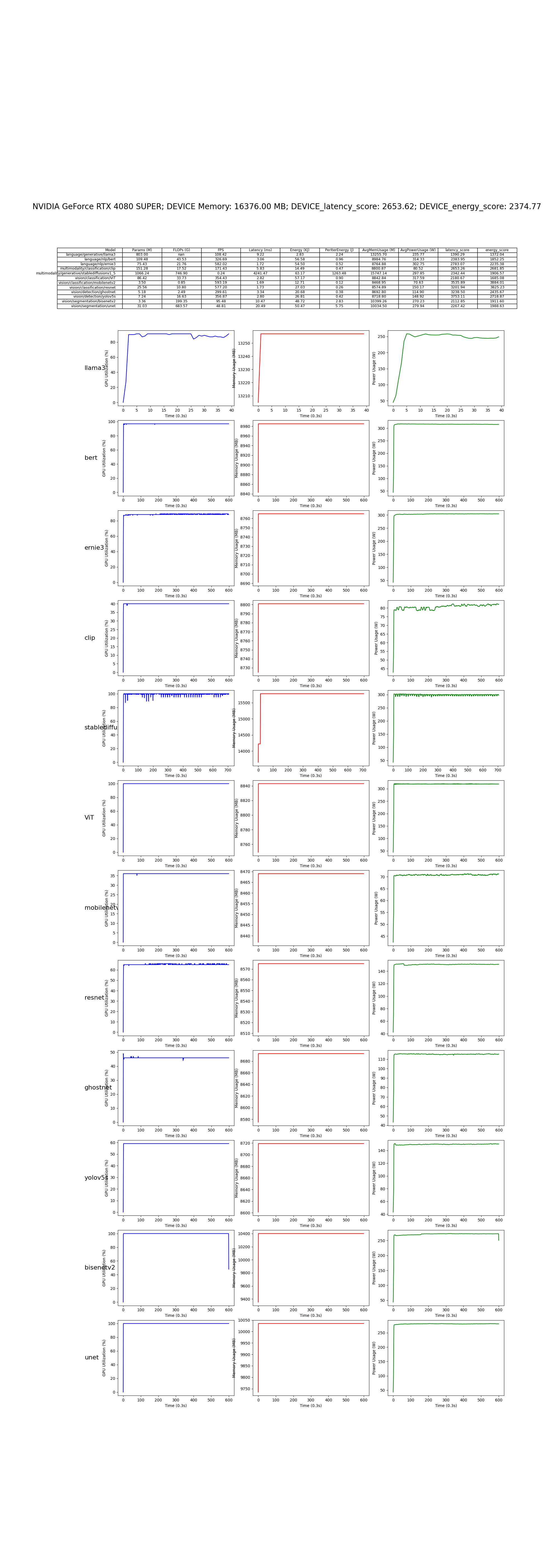
使用基于 PyTorch 的经典深度学习模型集合在 CUDA 平台上对 GPU NVIDIA 进行性能测试
仓库地址:AI-Benchmark-SDU
部分模型代码展示:
LLama3:
'''
Copyright (c) 2024, 山东大学智能创新研究院(Academy of Intelligent Innovation)

Redistribution and use in source and binary forms, with or without
modification, are permitted provided that the following conditions are met:

1. Redistributions of source code must retain the above copyright notice, this
   list of conditions and the following disclaimer.

2. Redistributions in binary form must reproduce the above copyright notice,
   this list of conditions and the following disclaimer in the documentation
   and/or other materials provided with the distribution.
'''
# Copyright (c) Academy of Intelligent Innovation.
# License-Identifier: BSD 2-Clause License
# AI Benchmark SDU Team

from model.model_set.model_base import BaseModel
from llama_cpp import Llama


class llama3_nvidia_amd(BaseModel):
    def __init__(self):
        super().__init__('language/generative/llama3')

    def get_input(self):
        self.input = "Q: Name the planets in the solar system? A: "

    def load_model(self):
        self.llm = Llama(
            model_path="model/model_set/pytorch/language/generative/llama3/ggml-meta-llama-3-8b-Q4_K_M.gguf",
            n_gpu_layers=99,
            #   n_gpu_layers=-1, # Uncomment to use GPU acceleration
            chat_format="llama-3",
            seed=1337, # Uncomment to set a specific seed
            n_ctx=2048, # Uncomment to increase the context window
            verbose=False
            )

    def get_params_flops(self) -> list:

        return [803, float('nan')]


    def inference(self):
        output = self.llm (
                prompt = self.input, # Prompt
                max_tokens=512, # Generate up to 32 tokens, set to None to generate up to the end of the context window
                stop=["Q:", "\n"], # Stop generating just before the model would generate a new question
                echo=True # Echo the prompt back in the output
            )
        completion_tokens = output['usage']['completion_tokens']
        return completion_tokens
CLIP:
'''
Copyright (c) 2024, 山东大学智能创新研究院(Academy of Intelligent Innovation)

Redistribution and use in source and binary forms, with or without
modification, are permitted provided that the following conditions are met:

1. Redistributions of source code must retain the above copyright notice, this
   list of conditions and the following disclaimer.

2. Redistributions in binary form must reproduce the above copyright notice,
   this list of conditions and the following disclaimer in the documentation
   and/or other materials provided with the distribution.
'''
# Copyright (c) Academy of Intelligent Innovation.
# License-Identifier: BSD 2-Clause License
# AI Benchmark SDU Team

import torch
from model.model_set.model_base import BaseModel
from model.model_set.models.multimodality.classification.clip.utils.model import build_model
from model.model_set.models.multimodality.classification.clip.utils.simpletokenizer import SimpleTokenizer as _Tokenizer
from thop import profile

class clip_nvidia_amd(BaseModel):
    def __init__(self):
        super().__init__('multimodality/classification/clip')

        self.text = ["a diagram", "a dog", "a cat"]
        self.input_shape =(1, 3, 224, 224)
        self.device = torch.device('cuda' if torch.cuda.is_available() else 'cpu')
        self.model_path = "model/model_set/pytorch/multimodality/classification/clip/ViT-B-32.pt"

    def get_input(self):
        self.img = torch.randn(self.input_shape).to(torch.float32).to(self.device)
        _tokenizer = _Tokenizer()
        sot_token = _tokenizer.encoder["<|startoftext|>"]
        eot_token = _tokenizer.encoder["<|endoftext|>"]
        all_tokens = [[sot_token] + _tokenizer.encode(text) + [eot_token] for text in self.text]
        context_length: int = 77
        truncate = False
        result = torch.zeros(len(all_tokens), context_length, dtype=torch.int)

        for i, tokens in enumerate(all_tokens):
            if len(tokens) > context_length:
                if truncate:
                    tokens = tokens[:context_length]
                    tokens[-1] = eot_token
                else:
                    raise RuntimeError(f"Input {self.text[i]} is too long for context length {context_length}")
            result[i, :len(tokens)] = torch.tensor(tokens)

        self.texts = result.to(self.device)

    def load_model(self):
        jit = False
        model = torch.jit.load(self.model_path, map_location=self.device if jit else "cpu").eval()
        state_dict = None
        self.model = build_model(state_dict or model.state_dict()).to(self.device)

    def get_params_flops(self) -> list:
        flops, _ = profile(self.model, (self.img, self.texts), verbose=False)
        params = sum(p.numel() for p in self.model.parameters() if p.requires_grad)
        return [flops / 1e9 * 2,  params / 1e6]

    def inference(self):
        image_features = self.model.encode_image(self.img)
        text_features = self.model.encode_text(self.texts)
        return image_features, text_features
在 NVIDIA GeForce RTX 4080 SUPER 上的测试结果:
OpenCL (NVIDIA)
OpenCL(Open Computing Language)是一个开放的、跨平台的并行计算框架。虽然NVIDIA主要推广其专有的CUDA平台,但它也支持OpenCL,为开发者提供了更多的灵活性和选择。
OpenCL 概述
-
开放标准:OpenCL由Khronos Group维护,是一个开放的行业标准。
-
跨平台:支持多种硬件,包括CPU、GPU、FPGA等。
-
异构计算:允许在不同类型的处理器上执行计算任务。
OpenCL 在 NVIDIA 平台上的特点
-
兼容性:NVIDIA的GPU驱动程序包含OpenCL实现,使得OpenCL程序可以在NVIDIA GPU上运行。
-
性能:虽然CUDA在NVIDIA硬件上可能提供更优化的性能,但OpenCL也能在NVIDIA GPU上实现高效的并行计算。
-
可移植性:使用OpenCL编写的程序可以在NVIDIA GPU以及其他厂商的硬件上运行,提供了更好的代码可移植性。
-
与CUDA的关系:OpenCL可以看作是CUDA的一个更通用的替代品,但在NVIDIA硬件上可能无法完全发挥其全部潜力。
OpenCL 架构
-
平台模型:包括一个主机和一个或多个OpenCL设备。
-
执行模型:
- 内核(Kernels):在OpenCL设备上执行的函数。
- 工作项(Work-items):内核的单个执行实例。
- 工作组(Work-groups):工作项的集合。
-
内存模型:定义了全局内存、常量内存、局部内存和私有内存。
-
编程模型:支持数据并行和任务并行。
OpenCL vs CUDA on NVIDIA
-
性能:CUDA通常在NVIDIA硬件上提供更好的性能,因为它是专门为NVIDIA GPU优化的。
-
开发工具:NVIDIA为CUDA提供更全面的开发工具和库支持。
-
学习曲线:OpenCL可能有更陡峭的学习曲线,因为它需要处理更多的硬件抽象。
-
市场份额:在NVIDIA生态系统中,CUDA更为普及。
虽然NVIDIA主要推广CUDA,但其对OpenCL的支持为开发者提供了另一种选择。OpenCL在NVIDIA平台上提供了良好的性能和跨平台兼容性,特别适合那些需要在多种硬件平台上运行的应用程序。然而,对于专门针对NVIDIA硬件优化的应用,CUDA可能是更好的选择。选择使用OpenCL还是CUDA取决于具体的项目需求、目标硬件平台和开发团队的专业知识。
技术栈架构
1. 系统软件层
- 设备驱动程序:
- 为特定硬件(如 GPU、CPU、FPGA)提供底层支持
- 实现 OpenCL 规范定义的功能
- 处理设备特定的优化和功能
- OpenCL ICD (Installable Client Driver):
- 提供对多个 OpenCL 实现的支持
- 允许在同一系统上共存多个 OpenCL 供应商的实现
- 管理不同 OpenCL 实现之间的切换和交互
2. 运行时环境层
- OpenCL Runtime:
- 提供 OpenCL API 的实现
- 管理设备、上下文、命令队列和内存对象
- 处理内核编译和执行
- 协调主机和设备之间的数据传输
- 支持事件和同步机制
3. 编程模型和语言层
- OpenCL C/C++:
- 基于 C99 标准的编程语言,用于编写 OpenCL 内核
- 支持向量数据类型和内置函数
- 提供内存模型和同步原语
- 允许编写可在各种设备上执行的并行代码
- OpenCL C++ 包装器:
- 为 C++ 程序员提供面向对象的 API
- 简化内存管理和错误处理
- 提供更现代的 C++ 接口
4. 计算库层
- clBLAS:
- OpenCL 实现的基本线性代数子程序(BLAS)库
- 提供矩阵和向量操作的高性能实现
- 支持多种设备类型
- clDNN (Compute Library for Deep Neural Networks):
- 用于深度学习的 OpenCL 加速库
- 提供常见的神经网络层和操作
- 优化for各种硬件平台
5. 框架模型层
- TensorFlow with OpenCL:
- 通过 ComputeCpp 或其他 OpenCL 后端支持 OpenCL
- 允许在支持 OpenCL 的设备上运行 TensorFlow 模型
- Caffe with OpenCL:
- 使用 OpenCL 后端的 Caffe 深度学习框架
- 支持在各种 OpenCL 设备上训练和推理
- OpenCV with OpenCL:
- 计算机视觉库,集成了 OpenCL 支持
- 利用 OpenCL 加速图像和视频处理操作
- ArrayFire:
- 高性能计算库,支持 OpenCL 后端
- 提供线性代数、信号处理和计算机视觉功能
- 简化了 OpenCL 编程,提供高级抽象
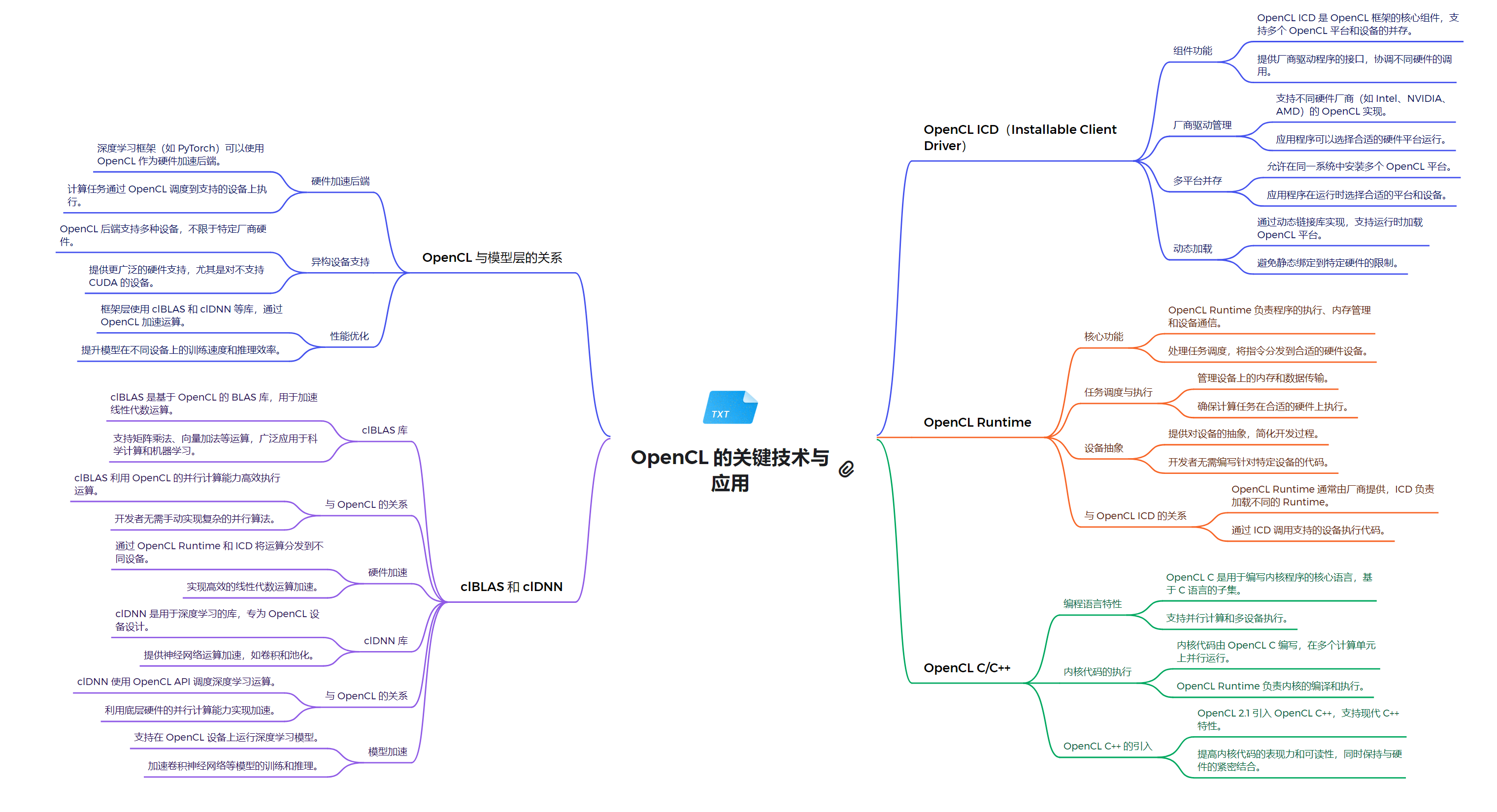
关系解析
OpenCL作为一个开放的异构计算框架,在模型层面支持硬件加速、跨设备兼容性和性能优化。它的核心组件包括OpenCL ICD、OpenCL Runtime和OpenCL C/C++语言。
OpenCL ICD (Installable Client Driver) 是一个关键组件,它允许多个OpenCL实现共存,提供了一个统一的接口来管理不同厂商的OpenCL实现。这种设计极大地增强了OpenCL的灵活性和可扩展性,使得开发者可以在不同的硬件平台上无缝切换。OpenCL Runtime负责管理设备、内存和任务调度等核心功能。它处理内存分配、数据传输、内核编译和执行等底层操作,为开发者提供了一个抽象层,简化了异构计算的复杂性。Runtime与ICD紧密协作,确保了OpenCL应用程序的高效运行。
在编程语言方面,OpenCL C/C++扩展了标准C/C++,增加了并行计算所需的特性。它支持向量数据类型、内存模型和并行编程构造,使得开发者能够充分利用异构计算资源。OpenCL 2.1引入了SPIR-V中间表示,进一步增强了跨平台兼容性和编译优化。clBLAS和clDNN是基于OpenCL的重要库,分别针对基础线性代数子程序和深度神经网络计算进行了优化。这些库充分利用了OpenCL的并行计算能力,为科学计算和机器学习应用提供了高性能解决方案。OpenCL与其他技术的集成也是其强大之处。例如,深度学习框架如PyTorch可以利用OpenCL进行GPU加速,而OpenCL本身也支持与CUDA等其他并行计算框架的互操作。
总的来说,OpenCL通过其灵活的架构、强大的运行时系统和丰富的编程接口,为异构计算提供了一个全面的解决方案。它不仅支持跨平台开发,还能够充分发挥各种计算设备的性能潜力,在高性能计算、图像处理、科学模拟等领域发挥着重要作用。OpenCL的生态系统持续发展,不断适应新的硬件架构和计算需求,为未来的并行计算和异构系统开发铺平了道路。
系统软件层
该程序使用OpenCL API 列出了系统中所有可用的 NVIDIA 设备,包括设备名称、驱动版本、计算单元数量和全局内存大小,并创建和销毁了一个OpenCL上下文。
-
获取OpenCL平台:使用
clGetPlatformIDs获取系统中的所有 OpenCL 平台。 -
检查NVIDIA平台:遍历平台列表,使用
clGetPlatformInfo检查是否为 NVIDIA 平台。 -
获取设备信息:通过
clGetDeviceIDs获取 NVIDIA 平台中的所有设备,并使用clGetDeviceInfo获取每个设备的详细信息,如设备名称、驱动版本和全局内存大小。 -
创建和销毁上下文:使用
clCreateContext创建一个 OpenCL 上下文,并在使用后释放该上下文。示例代码:
#include <iostream>
#include <cuda.h>

// Check the return value of CUDA functions and print error message on failure
void checkCudaErrors(CUresult result) {
    if (result != CUDA_SUCCESS) {
        const char *errorStr;
        cuGetErrorString(result, &errorStr);
        std::cerr << "CUDA Error: " << errorStr << std::endl;
        exit(EXIT_FAILURE);
    }
}

// Print information about a CUDA device
void printDeviceInfo(CUdevice device) {
    int driverVersion = 0;
    char deviceName[256];
    // Get device name
    checkCudaErrors(cuDeviceGetName(deviceName, sizeof(deviceName), device));

    int computeCapabilityMajor, computeCapabilityMinor;
    // Get the major and minor version of compute capability
    checkCudaErrors(cuDeviceGetAttribute(&computeCapabilityMajor, CU_DEVICE_ATTRIBUTE_COMPUTE_CAPABILITY_MAJOR, device));
    checkCudaErrors(cuDeviceGetAttribute(&computeCapabilityMinor, CU_DEVICE_ATTRIBUTE_COMPUTE_CAPABILITY_MINOR, device));

    size_t totalGlobalMem;
    checkCudaErrors(cuDeviceTotalMem(&totalGlobalMem, device));
    checkCudaErrors(cuDriverGetVersion(&driverVersion));

    // Print device details
    std::cout << "Device Name: " << deviceName << std::endl;
    std::cout << "Compute Capability: " << computeCapabilityMajor << "." << computeCapabilityMinor << std::endl;
    std::cout << "CUDA Driver Version: " << driverVersion / 1000 << "." << (driverVersion % 100) / 10 << std::endl;
    std::cout << "Total Global Memory: " << totalGlobalMem / (1024 * 1024) << " MB" << std::endl;
}

int main() {
    // Initialize CUDA
    checkCudaErrors(cuInit(0));

    // Get the number of available CUDA devices
    int deviceCount;
    checkCudaErrors(cuDeviceGetCount(&deviceCount));
    std::cout << "Number of CUDA Devices: " << deviceCount << std::endl;

    CUdevice device;
    // Iterate through each device and print its information
    for (int i = 0; i < deviceCount; i++) {
        checkCudaErrors(cuDeviceGet(&device, i));
        printDeviceInfo(device);
        std::cout << std::endl;
    }

    CUcontext context;
    // Create a CUDA context and set it as the current context
    checkCudaErrors(cuCtxCreate(&context, 0, deviceCount > 0 ? device : 0));
    checkCudaErrors(cuCtxSetCurrent(context));

    std::cout << "CUDA context created successfully." << std::endl;

    checkCudaErrors(cuCtxDestroy(context));

    return 0;
}
结果:
Platform Name: NVIDIA CUDA
Device Name: NVIDIA GeForce RTX 4080 SUPER
Driver Version: 550.107.02
Max Compute Units: 80
Global Memory Size: 16072 MB

OpenCL context created successfully.
运行时环境层
OpenCL Runtime 是一个软件组件,负责在不同平台和硬件设备上执行 OpenCL 程序。它提供了一系列 API 和工具,帮助开发者管理计算设备、创建和编译 OpenCL 程序、调度任务以及进行内存管理。
设备管理:负责发现和管理可用的计算设备(如 CPU、GPU、FPGA 等),并提供接口以查询设备属性;
上下文创建:用于创建和管理 OpenCL 上下文,上下文包含了设备、内存对象、命令队列和程序;
内存管理:提供内存分配和管理功能,包括在设备上分配和释放内存,支持主机与设备之间的数据传输;
程序编译与执行:支持从源代码创建程序对象,并编译为设备可执行的代码。同时负责调度和执行内核;
命令队列管理:提供命令队列的创建和管理功能,允许用户异步地提交计算任务;
事件和同步:处理事件和同步机制,以确保内核和数据传输的正确顺序执行;
代码示例如下:
#define CL_TARGET_OPENCL_VERSION 220
#include <CL/cl.h>
#include <stdio.h>
#include <stdlib.h>
#include <cstring>


#define ARRAY_SIZE 1024

// OpenCL kernel code for vector addition
const char* kernelSource = "__kernel void vec_add(__global float* A, __global float* B, __global float* C) { \
                                int id = get_global_id(0); \
                                C[id] = A[id] + B[id]; \
                            }";

int main() {
    cl_platform_id platform_id;
    cl_device_id device_id;
    cl_context context;
    cl_command_queue queue;
    cl_program program;
    cl_kernel kernel;
    cl_int ret;

    // Arrays on the host
    float A[ARRAY_SIZE], B[ARRAY_SIZE], C[ARRAY_SIZE];
    for (int i = 0; i < ARRAY_SIZE; i++) {
        A[i] = i;
        B[i] = i * 2;
    }

    // 1. Get the number of platforms
    cl_uint num_platforms;
    ret = clGetPlatformIDs(0, NULL, &num_platforms);
    if (ret != CL_SUCCESS) {
        printf("Failed to get platform IDs\n");
        return -1;
    }

    cl_platform_id* platforms = (cl_platform_id*)malloc(num_platforms * sizeof(cl_platform_id));
    ret = clGetPlatformIDs(num_platforms, platforms, NULL);
    if (ret != CL_SUCCESS) {
        printf("Failed to get platforms\n");
        free(platforms);
        return -1;
    }

    // Try to find the NVIDIA platform
    for (cl_uint i = 0; i < num_platforms; i++) {
        char platform_name[128];
        clGetPlatformInfo(platforms[i], CL_PLATFORM_NAME, sizeof(platform_name), platform_name, NULL);
        printf("Platform %d: %s\n", i, platform_name);

        if (strstr(platform_name, "NVIDIA") != NULL) {
            platform_id = platforms[i];
            printf("Selected NVIDIA platform: %s\n", platform_name);
            break;
        }
    }

    if (!platform_id) {
        printf("NVIDIA platform not found\n");
        free(platforms);
        return -1;
    }

    // 2. Get the GPU device from the selected NVIDIA platform
    ret = clGetDeviceIDs(platform_id, CL_DEVICE_TYPE_GPU, 1, &device_id, NULL);
    if (ret != CL_SUCCESS) {
        printf("Failed to get GPU device ID from NVIDIA platform, error code: %d\n", ret);
        free(platforms);
        return -1;
    }

    // Print the selected device
    char device_name[128];
    clGetDeviceInfo(device_id, CL_DEVICE_NAME, sizeof(device_name), device_name, NULL);
    printf("Selected device: %s\n", device_name);

    // 3. Create a context
    context = clCreateContext(NULL, 1, &device_id, NULL, NULL, &ret);
    if (ret != CL_SUCCESS) {
        printf("Failed to create context\n");
        free(platforms);
        return -1;
    }
    printf("Context created successfully.\n");

    // 4. Create a command queue
    queue = clCreateCommandQueueWithProperties(context, device_id, 0, &ret);
    if (ret != CL_SUCCESS) {
        printf("Failed to create command queue\n");
        free(platforms);
        return -1;
    }
    printf("Command queue created successfully.\n");

    // 5. Create a program from the kernel source
    program = clCreateProgramWithSource(context, 1, &kernelSource, NULL, &ret);
    if (ret != CL_SUCCESS) {
        printf("Failed to create program\n");
        free(platforms);
        return -1;
    }
    printf("Program created successfully.\n");

    // 6. Build the program
    ret = clBuildProgram(program, 1, &device_id, NULL, NULL, NULL);
    if (ret != CL_SUCCESS) {
        printf("Failed to build program\n");
        char log[1024];
        clGetProgramBuildInfo(program, device_id, CL_PROGRAM_BUILD_LOG, sizeof(log), log, NULL);
        printf("Build log:\n%s\n", log);
        free(platforms);
        return -1;
    }
    printf("Program built successfully.\n");

    // 7. Create the kernel
    kernel = clCreateKernel(program, "vec_add", &ret);
    if (ret != CL_SUCCESS) {
        printf("Failed to create kernel\n");
        free(platforms);
        return -1;
    }
    printf("Kernel created successfully.\n");

    // 8. Create buffers for the input and output arrays
    cl_mem buffer_A = clCreateBuffer(context, CL_MEM_READ_ONLY, ARRAY_SIZE * sizeof(float), NULL, &ret);
    cl_mem buffer_B = clCreateBuffer(context, CL_MEM_READ_ONLY, ARRAY_SIZE * sizeof(float), NULL, &ret);
    cl_mem buffer_C = clCreateBuffer(context, CL_MEM_WRITE_ONLY, ARRAY_SIZE * sizeof(float), NULL, &ret);

    if (ret != CL_SUCCESS) {
        printf("Failed to create buffers\n");
        free(platforms);
        return -1;
    }
    printf("Buffers created successfully.\n");

    // 9. Copy the input data to the respective memory buffers
    ret = clEnqueueWriteBuffer(queue, buffer_A, CL_TRUE, 0, ARRAY_SIZE * sizeof(float), A, 0, NULL, NULL);
    ret |= clEnqueueWriteBuffer(queue, buffer_B, CL_TRUE, 0, ARRAY_SIZE * sizeof(float), B, 0, NULL, NULL);
    if (ret != CL_SUCCESS) {
        printf("Failed to write to buffers\n");
        free(platforms);
        return -1;
    }
    printf("Data written to buffers successfully.\n");

    // 10. Set the kernel arguments
    ret = clSetKernelArg(kernel, 0, sizeof(cl_mem), (void*)&buffer_A);
    ret |= clSetKernelArg(kernel, 1, sizeof(cl_mem), (void*)&buffer_B);
    ret |= clSetKernelArg(kernel, 2, sizeof(cl_mem), (void*)&buffer_C);
    if (ret != CL_SUCCESS) {
        printf("Failed to set kernel arguments\n");
        free(platforms);
        return -1;
    }
    printf("Kernel arguments set successfully.\n");

    // 11. Execute the kernel
    size_t global_size = ARRAY_SIZE;
    ret = clEnqueueNDRangeKernel(queue, kernel, 1, NULL, &global_size, NULL, 0, NULL, NULL);
    if (ret != CL_SUCCESS) {
        printf("Failed to enqueue kernel\n");
        free(platforms);
        return -1;
    }
    printf("Kernel enqueued successfully.\n");

    // 12. Read the output buffer back to the host
    ret = clEnqueueReadBuffer(queue, buffer_C, CL_TRUE, 0, ARRAY_SIZE * sizeof(float), C, 0, NULL, NULL);
    if (ret != CL_SUCCESS) {
        printf("Failed to read from buffer\n");
        free(platforms);
        return -1;
    }
    printf("Data read from buffer successfully.\n");

    // Output the results
    printf("Result:\n");
    for (int i = 0; i < 10; i++) {
        printf("C[%d] = %f\n", i, C[i]);
    }

    // 13. Clean up
    clReleaseMemObject(buffer_A);
    clReleaseMemObject(buffer_B);
    clReleaseMemObject(buffer_C);
    clReleaseKernel(kernel);
    clReleaseProgram(program);
    clReleaseCommandQueue(queue);
    clReleaseContext(context);
    free(platforms);

    printf("Resources released successfully.\n");
    return 0;
}
结果:
Platform 0: Intel(R) OpenCL
Platform 1: NVIDIA CUDA
Selected NVIDIA platform: NVIDIA CUDA
Selected device: NVIDIA GeForce RTX 4080 SUPER
Context created successfully.
Command queue created successfully.
Program created successfully.
Program built successfully.
Kernel created successfully.
Buffers created successfully.
Data written to buffers successfully.
Kernel arguments set successfully.
Kernel enqueued successfully.
Data read from buffer successfully.
Result:
C[0] = 0.000000
C[1] = 3.000000
C[2] = 6.000000
C[3] = 9.000000
C[4] = 12.000000
C[5] = 15.000000
C[6] = 18.000000
C[7] = 21.000000
C[8] = 24.000000
C[9] = 27.000000
结果说明:
Platform 0: Intel(R) OpenCL
表示系统上检测到一个 OpenCL 平台,提供商是 Intel,可能是用于 CPU 或集成显卡的 OpenCL 运行时;
Platform 1: NVIDIA CUDA
表示另一个 OpenCL 平台由 NVIDIA 提供,基于 CUDA 技术,能够在 NVIDIA GPU 上运行 OpenCL 程序;
Selected NVIDIA platform: NVIDIA CUDA
程序成功选择了 NVIDIA CUDA 平台,以在 NVIDIA GPU 上运行;
Selected device: NVIDIA GeForce RTX 4080 SUPER
选择的设备是 NVIDIA GeForce RTX 4080 SUPER,这是你的 GPU,程序将在此设备上执行计算;
Context created successfully.
成功创建了 OpenCL 上下文(context),它负责管理设备、内核和内存对象的生命周期;
Command queue created successfully.
成功创建了命令队列,程序通过此队列向 GPU 发送计算任务;
Program created successfully.
OpenCL 程序(从字符串中创建)已成功创建。该程序包含内核代码;
Program built successfully.
内核程序已成功编译和构建,没有语法或其他构建错误;
Kernel created successfully.
程序中定义的内核函数 hello 成功创建,可以在设备上运行;
Buffers created successfully.
程序成功为 GPU 分配了缓冲区(内存对象),这些缓冲区将用于存储输入数据和输出结果;
Data written to buffers successfully.
输入数据已经成功写入 GPU 缓冲区,准备进行计算;
Kernel arguments set successfully.
成功将内核函数的参数设置为相应的 GPU 缓冲区;
Kernel enqueued successfully.
内核已被添加到命令队列中,准备在 GPU 上执行;
Data read from buffer successfully.
内核执行完成后,成功从 GPU 缓冲区中读取结果数据;
Result:
C[0] = 0.000000
C[1] = 3.000000
C[2] = 6.000000
C[3] = 9.000000
C[4] = 12.000000
C[5] = 15.000000
C[6] = 18.000000
C[7] = 21.000000
C[8] = 24.000000
C[9] = 27.000000
这是计算结果,可能是一个简单的线性计算,每个输出值是由内核函数计算得到的。此例中,每个结果都以步长 3 递增,从 0 开始;
Resources released successfully.
程序成功释放了所有分配的资源,包括内核、程序、队列、上下文等。
编程模型和语言层
OpenCL 支持在多种设备上进行并行计算,如CPU、GPU、FPGA等。OpenCL 由 Khronos Group 管理,是一种跨平台的并行编程语言,它在不同的硬件架构上提供了统一的编程接口。
1. OpenCL 的核心编程特性
OpenCL 是一个相对底层的 API,与 CUDA 类似,它同样强调对设备内存和计算资源的精确控制。OpenCL的编程模型包含以下关键特性:
- 平台模型 :OpenCL 的平台模型由 主机(host) 和一个或多个 设备(device) 组成。在一个平台上,主机通常是 CPU,设备可以是 GPU 或其他加速器。开发者需要显式地管理主机和设备之间的交互。
- 上下文和命令队列 :OpenCL 引入了上下文(context)来管理设备,程序对象和内存对象的生命周期。命令队列(command queue)用于调度执行内核(kernel)和数据传输操作。每个设备都拥有一个或多个命令队列,支持并行化任务执行。
- 内核(Kernel)函数 :OpenCL 的计算核心是内核函数,它定义了在设备上并行执行的代码。内核函数使用
__kernel修饰符,表明其在设备上执行。内核的执行由全局工作项(global work-items)和局部工作组(local work-groups)组织。
__kernel void vectorAdd(__global const float* A, __global const float* B, __global float* C, int N) {
    int i = get_global_id(0);
    if (i < N) C[i] = A[i] + B[i];
}
这个简单的内核展示了如何通过OpenCL执行并行向量加法运算,get_global_id(0) 获取当前工作项的唯一ID,用于计算索引。
- 内存模型 :OpenCL 的内存模型包括全局内存(global memory)、常量内存(constant memory)、局部内存(local memory)和私有内存(private memory)。每个工作项可以访问不同级别的内存,这些内存具有不同的性能特性和作用范围。
- 设备和内存管理 :与CUDA类似,OpenCL要求开发者手动管理主机和设备之间的内存传输。通过
clCreateBuffer创建缓冲区对象,并使用clEnqueueWriteBuffer和clEnqueueReadBuffer在主机和设备之间传输数据。
2. 算子编写示例:矩阵乘法
矩阵乘法是并行计算中常见的操作之一,下面展示如何在OpenCL中实现并行矩阵乘法:
__kernel void matrixMul(__global float* A, __global float* B, __global float* C, int N) {
    int row = get_global_id(1);
    int col = get_global_id(0);
    float result = 0.0;
    if (row < N && col < N) {
        for (int i = 0; i < N; ++i) {
            result += A[row * N + i] * B[i * N + col];
        }
        C[row * N + col] = result;
    }
}
该内核函数中,使用 get_global_id(0) 和 get_global_id(1) 分别获取当前工作项在全局工作空间中的横纵坐标(行和列)。每个工作项负责计算结果矩阵中的一个元素,通过访问内存中的数据并进行并行计算实现。
3. 并行计算模型介绍
OpenCL 的并行计算模型与 CUDA 在一些方面类似,但它是一个更加通用的异构计算标准,能够在不同的硬件架构上执行。以下是 OpenCL 并行计算模型的主要概念:
- 工作项(Work-Item)与工作组(Work-Group) :OpenCL 中的并行计算任务被划分为工作项,每个工作项独立执行一小部分计算。多个工作项组成工作组,工作组之间相互独立,工作项可以在同一工作组中共享数据并进行同步操作。
- 全局与局部内存 :工作项可以访问全局内存,但全局内存通常比局部内存慢。因此,合理使用局部内存来减少对全局内存的访问可以极大提升性能。
- 命令队列与同步 :在OpenCL中,主机通过命令队列向设备提交计算任务。OpenCL支持事件机制,允许在任务完成后触发事件。这种机制使得开发者可以更好地控制任务的调度和设备的计算资源。
4. OpenCL 与 CUDA 的对比
虽然 OpenCL 和 CUDA 在设计上有一些相似之处,特别是在内存模型和并行任务调度方面,但它们之间仍然存在显著差异:
- 跨平台性 :CUDA 是 NVIDIA 专有的技术,虽然在 NVIDIA GPU 上表现优异,但只能用于 NVIDIA 硬件。相比之下,OpenCL 是一个跨平台标准,支持在各种硬件上执行,适合需要在多种设备上运行的异构计算场景。
- 生态与性能 :虽然 OpenCL 提供了跨平台的灵活性,但由于其底层抽象程度较高,性能在某些情况下可能不及 CUDA 尤其是在 NVIDIA 硬件上。NVIDIA 对 CUDA 的优化力度更大,提供了许多额外的库支持(如 cuBLAS、cuDNN),而这些库在 OpenCL 上并不可用。
- 编程复杂度 :OpenCL 代码编写通常较为复杂,因为它需要显式管理设备上下文、内存分配、内核调度等。而 CUDA 通过一些简化的工具和库,使得编程过程相对更加简便。
5. OpenCL 在 AI 开发中的应用
尽管 OpenCL 在深度学习和AI开发中的应用不如CUDA广泛,但它在某些特定的场景下仍然具有重要的价值,尤其是那些需要跨平台计算的环境:
- 通用性和兼容性 :对于那些需要在不同硬件平台上运行的AI应用,OpenCL 提供了跨平台的并行计算支持。例如,在一些需要同时支持CPU和AMD、NVIDIA GPU的场景中,OpenCL的兼容性使得它成为理想的选择。
- 嵌入式与低功耗设备 :在边缘计算和嵌入式设备中,OpenCL 因为其广泛的硬件支持,能够在资源有限的环境中提供GPU加速能力。
- 优化深度学习库 :虽然NVIDIA更多推崇CUDA,但像 ARM、AMD 等厂商在其AI硬件上更多依赖OpenCL,推动了在这些平台上对深度学习库(如 TensorFlow Lite 和 ONNX Runtime)的优化。
6. 总结
NVIDIA OpenCL 提供了一套灵活的并行编程模型,适合跨平台的异构计算场景。在 NVIDIA 平台上,尽管 CUDA 是更加成熟的选择,但 OpenCL 作为通用的并行编程标准,依然在一些跨平台应用和异构计算中具有重要地位。通过理解 OpenCL 的编程模型,开发者能够在需要跨设备和跨平台的应用中充分发挥其优势,构建高效的并行计算系统。
计算库层
clBLAS 是一个开源的高性能线性代数库,专为 OpenCL 平台设计,支持多种基本线性代数操作,如矩阵乘法和矩阵-向量乘法。clBLAS 利用 OpenCL 的并行计算能力,提供灵活的内存管理和高效的内核优化,显著提升线性代数运算的性能。
参考仓库地址:clBLAS
clblasChemm 展示了如何使用 clBLAS 进行复数矩阵的乘法操作。
示例代码如下:
/* ************************************************************************
 * Copyright 2013 Advanced Micro Devices, Inc.
 *
 * Licensed under the Apache License, Version 2.0 (the "License");
 * you may not use this file except in compliance with the License.
 * You may obtain a copy of the License at
 *
 * http://www.apache.org/licenses/LICENSE-2.0
 *
 * Unless required by applicable law or agreed to in writing, software
 * distributed under the License is distributed on an "AS IS" BASIS,
 * WITHOUT WARRANTIES OR CONDITIONS OF ANY KIND, either express or implied.
 * See the License for the specific language governing permissions and
 * limitations under the License.
 * ************************************************************************/


#include <sys/types.h>
#include <stdio.h>
#include <string.h>

/* Include CLBLAS header. It automatically includes needed OpenCL header,
 * so we can drop out explicit inclusion of cl.h header.
 */
#include <clBLAS.h>

/* This example uses predefined matrices and their characteristics for
 * simplicity purpose.
 */
static const clblasOrder order = clblasRowMajor;

#define M  4
#define N  3

static const cl_float2 alpha = {{10, 10}};

static const clblasSide side = clblasLeft;
static const clblasUplo uplo = clblasLower;
static const cl_float2 A[M*M] = {
    {{11, 12}}, {{-1, -1}}, {{-1, -1}}, {{-1, -1}},
    {{21, 22}}, {{22, 23}}, {{-1, -1}}, {{-1, -1}},
    {{31, 32}}, {{32, 33}}, {{33, 34}}, {{-1, -1}},
    {{41, 61}}, {{42, 62}}, {{43, 73}}, {{44, 23}}
};
static const size_t lda = M;

static const cl_float2 B[M*N] = {
    {{11, -21}},  {{-12, 23}}, {{13, 33}},
    {{21, 12}},   {{22, -10}}, {{23, 5}},
    {{31, 1}},    {{-32, 65}}, {{33, -1}},
    {{1, 41}},    {{-33, 42}}, {{12, 43}},
};
static const size_t ldb = N;

static const cl_float2 beta = {{20, 20}};

static cl_float2 C[M*N] = {
    {{11, 11}},  {{-12, 12}}, {{13, 33}},
    {{21, -32}}, {{22,  -1}}, {{23, 0}},
    {{31, 13}},  {{-32, 78}}, {{33, 45}},
    {{41, 14}},  {{0,   42}}, {{43, -1}},
};
static const size_t ldc = N;

static void
printResult(void)
{
    size_t i, j, nrows;

    printf("Result:\n");

    nrows = (sizeof(C) / sizeof(cl_float2)) / ldc;
    for (i = 0; i < nrows; i++) {
        for (j = 0; j < ldc; j++) {
            printf("<%9.2f, %-9.2f> ", CREAL(C[i * ldc + j]), CIMAG(C[i*ldc + j]));
        }
        printf("\n");
    }
}

int
main(void)
{
    cl_int err;
    cl_platform_id platform = 0;
    cl_device_id device = 0;
    cl_context_properties props[3] = { CL_CONTEXT_PLATFORM, 0, 0 };
    cl_context ctx = 0;
    cl_command_queue queue = 0;
    cl_mem bufA, bufB, bufC;
    cl_event event = NULL;
    int ret = 0;

    /* Setup OpenCL environment. */
    err = clGetPlatformIDs(1, &platform, NULL);
    if (err != CL_SUCCESS) {
        printf( "clGetPlatformIDs() failed with %d\n", err );
        return 1;
    }

    err = clGetDeviceIDs(platform, CL_DEVICE_TYPE_GPU, 1, &device, NULL);
    if (err != CL_SUCCESS) {
        printf( "clGetDeviceIDs() failed with %d\n", err );
        return 1;
    }

    props[1] = (cl_context_properties)platform;
    ctx = clCreateContext(props, 1, &device, NULL, NULL, &err);
    if (err != CL_SUCCESS) {
        printf( "clCreateContext() failed with %d\n", err );
        return 1;
    }

    queue = clCreateCommandQueue(ctx, device, 0, &err);
    if (err != CL_SUCCESS) {
        printf( "clCreateCommandQueue() failed with %d\n", err );
        clReleaseContext(ctx);
        return 1;
    }

    /* Setup clblas. */
    err = clblasSetup();
    if (err != CL_SUCCESS) {
        printf("clblasSetup() failed with %d\n", err);
        clReleaseCommandQueue(queue);
        clReleaseContext(ctx);
        return 1;
    }

    /* Prepare OpenCL memory objects and place matrices inside them. */
    bufA = clCreateBuffer(ctx, CL_MEM_READ_ONLY, M * M * sizeof(*A),
                          NULL, &err);
    bufB = clCreateBuffer(ctx, CL_MEM_READ_ONLY, M * N * sizeof(*B),
                          NULL, &err);
    bufC = clCreateBuffer(ctx, CL_MEM_READ_WRITE, M * N * sizeof(*C),
                          NULL, &err);

    err = clEnqueueWriteBuffer(queue, bufA, CL_TRUE, 0,
        M * M * sizeof(*A), A, 0, NULL, NULL);
    err = clEnqueueWriteBuffer(queue, bufB, CL_TRUE, 0,
        M * N * sizeof(*B), B, 0, NULL, NULL);
    err = clEnqueueWriteBuffer(queue, bufC, CL_TRUE, 0,
        M * N * sizeof(*C), C, 0, NULL, NULL);

    /* Call clblas function. */
    err = clblasChemm(order, side, uplo, M, N, alpha, bufA,
                         0, lda, bufB, 0, ldb, beta, bufC, 0, ldc, 1, &queue,
                         0, NULL, &event);
    if (err != CL_SUCCESS) {
        printf("clblasSsymm() failed with %d\n", err);
        ret = 1;
    }
    else {
        /* Wait for calculations to be finished. */
        err = clWaitForEvents(1, &event);

        /* Fetch results of calculations from GPU memory. */
        err = clEnqueueReadBuffer(queue, bufC, CL_TRUE, 0, M * N * sizeof(*C),
                                  C, 0, NULL, NULL);

        /* At this point you will get the result of SYMM placed in C array. */
        printResult();
    }

    /* Release OpenCL events. */
    clReleaseEvent(event);

    /* Release OpenCL memory objects. */
    clReleaseMemObject(bufC);
    clReleaseMemObject(bufB);
    clReleaseMemObject(bufA);

    /* Finalize work with clblas. */
    clblasTeardown();

    /* Release OpenCL working objects. */
    clReleaseCommandQueue(queue);
    clReleaseContext(ctx);

    return ret;
}
结果:
Result:
< 41430.00, 46230.00 > <-39740.00, 87400.00 > < 48960.00, 48400.00 >
< 41360.00, 54760.00 > <-48340.00, 90520.00 > < 32620.00, 53220.00 >
< 28830.00, 79370.00 > <-67980.00, 77040.00 > < 13400.00, 81160.00 >
<-24980.00, 90100.00 > <-114700.00, -43780.00> <-67560.00, 93200.00 >
clblasScopy 是 clBLAS 库中的一个函数,它是 BLAS 标准中 scopy 函数的 OpenCL 版本。scopy 函数的作用是复制浮点数组。在 clBLAS 中,clblasScopy 用于将一个浮点数组复制到另一个浮点数组,这两个数组可以位于不同的内存区域。
示例代码如下:
/* ************************************************************************
 * Copyright 2013 Advanced Micro Devices, Inc.
 *
 * Licensed under the Apache License, Version 2.0 (the "License");
 * you may not use this file except in compliance with the License.
 * You may obtain a copy of the License at
 *
 * http://www.apache.org/licenses/LICENSE-2.0
 *
 * Unless required by applicable law or agreed to in writing, software
 * distributed under the License is distributed on an "AS IS" BASIS,
 * WITHOUT WARRANTIES OR CONDITIONS OF ANY KIND, either express or implied.
 * See the License for the specific language governing permissions and
 * limitations under the License.
 * ************************************************************************/

#include <sys/types.h>
#include <stdio.h>
#include <string.h>
#include <math.h>

/* Include CLBLAS header. It automatically includes needed OpenCL header,
 * so we can drop out explicit inclusion of cl.h header.
 */
#include <clBLAS.h>

/* This example uses predefined matrices and their characteristics for
 * simplicity purpose.
 */
static const size_t N = 7;
static cl_float X[] = {
    11,
    21,
    31,
    41,
    51,
    61,
    71,
};
static const int incx = 1;

static cl_float Y[] = {
    0,
    2,
    0,
    0,
    0,
    5,
    0,
};
static const int incy = 1;


static void
printResult(void)
{
    size_t i;
    printf("\nResult:\n");

    printf(" X\n");
    for (i = 0; i < N; i++) {
            printf("\t%f\n", X[i]);
    }

    printf("Y\n");
    for (i = 0; i < N; i++) {
            printf("\t%f\n", Y[i]);
    }
}

int
main(void)
{
    cl_int err;
    cl_platform_id platform = 0;
    cl_device_id device = 0;
    cl_context_properties props[3] = { CL_CONTEXT_PLATFORM, 0, 0 };
    cl_context ctx = 0;
    cl_command_queue queue = 0;
    cl_mem bufX, bufY;
    cl_event event = NULL;
    int ret = 0;
    int lenX = 1 + (N-1)*abs(incx);
    int lenY = 1 + (N-1)*abs(incy);

    /* Setup OpenCL environment. */
    err = clGetPlatformIDs(1, &platform, NULL);
    if (err != CL_SUCCESS) {
        printf( "clGetPlatformIDs() failed with %d\n", err );
        return 1;
    }

    err = clGetDeviceIDs(platform, CL_DEVICE_TYPE_GPU, 1, &device, NULL);
    if (err != CL_SUCCESS) {
        printf( "clGetDeviceIDs() failed with %d\n", err );
        return 1;
    }

    props[1] = (cl_context_properties)platform;
    ctx = clCreateContext(props, 1, &device, NULL, NULL, &err);
    if (err != CL_SUCCESS) {
        printf( "clCreateContext() failed with %d\n", err );
        return 1;
    }

    queue = clCreateCommandQueue(ctx, device, 0, &err);
    if (err != CL_SUCCESS) {
        printf( "clCreateCommandQueue() failed with %d\n", err );
        clReleaseContext(ctx);
        return 1;
    }

    /* Setup clblas. */
    err = clblasSetup();
    if (err != CL_SUCCESS) {
        printf("clblasSetup() failed with %d\n", err);
        clReleaseCommandQueue(queue);
        clReleaseContext(ctx);
        return 1;
    }

    /* Prepare OpenCL memory objects and place matrices inside them. */
    bufX = clCreateBuffer(ctx, CL_MEM_READ_ONLY, (lenX*sizeof(cl_float)), NULL, &err);
    bufY = clCreateBuffer(ctx, CL_MEM_READ_WRITE, (lenY*sizeof(cl_float)), NULL, &err);

    err = clEnqueueWriteBuffer(queue, bufX, CL_TRUE, 0, (lenX*sizeof(cl_float)), X, 0, NULL, NULL);
    err = clEnqueueWriteBuffer(queue, bufY, CL_TRUE, 0, (lenY*sizeof(cl_float)), Y, 0, NULL, NULL);

    /* Call clblas function. */
    err = clblasScopy( N, bufX, 0, incx, bufY, 0, incy, 1, &queue, 0, NULL, &event);
    if (err != CL_SUCCESS) {
        printf("clblasScopy() failed with %d\n", err);
        ret = 1;
    }
    else {
        /* Wait for calculations to be finished. */
        err = clWaitForEvents(1, &event);

        /* Fetch results of calculations from GPU memory. */
        err = clEnqueueReadBuffer(queue, bufX, CL_TRUE, 0, (lenX*sizeof(cl_float)),
                                    X, 0, NULL, NULL);
        err = clEnqueueReadBuffer(queue, bufY, CL_TRUE, 0, (lenY*sizeof(cl_float)),
                                    Y, 0, NULL, NULL);

        /* At this point you will get the result of SSWAP placed in vector Y. */
        printResult();
    }

    /* Release OpenCL events. */
    clReleaseEvent(event);

    /* Release OpenCL memory objects. */
    clReleaseMemObject(bufY);
    clReleaseMemObject(bufX);

    /* Finalize work with clblas. */
    clblasTeardown();

    /* Release OpenCL working objects. */
    clReleaseCommandQueue(queue);
    clReleaseContext(ctx);

    return ret;
}
结果:
Result:
 X
        11.000000
        21.000000
        31.000000
        41.000000
        51.000000
        61.000000
        71.000000
Y
        11.000000
        21.000000
        31.000000
        41.000000
        51.000000
        61.000000
        71.000000
clblasSgemm 是 clBLAS 库中的一个函数,用于执行单精度浮点数的矩阵乘法。Sgemm 代表单精度(Single precision)和矩阵乘法(GEneral Matrix-Matrix multiplication)。这个函数是 BLAS 库中最基本的函数之一,广泛用于科学计算、工程模拟、数据分析和机器学习等领域。
示例代码如下:
#include <stdio.h>
#include <stdlib.h>
#include <CL/cl.h>
#include <clBLAS.h>
#include <sys/time.h>

#define M 320
#define N 320
#define K 320
#define ITERATIONS 300

static const clblasOrder order = clblasRowMajor;
static const cl_float alpha = 1.0f;
static const clblasTranspose transA = clblasNoTrans;
static const clblasTranspose transB = clblasNoTrans;
static const cl_float beta = 0.0f;

static cl_float A[M*K];
static cl_float B[K*N];
static cl_float C[M*N];
static cl_float result[M*N];

void initMatrix(cl_float *mat, size_t size, cl_float value) {
    for (size_t i = 0; i < size; i++) {
        mat[i] = value;
    }
}

double getCurrentTimeInMilliseconds() {
    struct timeval time;
    gettimeofday(&time, NULL);
    return time.tv_sec * 1000.0 + time.tv_usec / 1000.0;
}

int main(void) {
    cl_int err;
    cl_platform_id platform = 0;
    cl_device_id device = 0;
    cl_context_properties props[3] = { CL_CONTEXT_PLATFORM, 0, 0 };
    cl_context ctx = 0;
    cl_command_queue queue = 0;
    cl_mem bufA, bufB, bufC;
    cl_event event = NULL;

    printf("[Matrix Multiply Using clBLAS] - Starting...\n");

    // Initialize matrices
    initMatrix(A, M * K, 1.0f);
    initMatrix(B, K * N, 0.01f);
    initMatrix(C, M * N, 0.0f);

    // Setup OpenCL environment
    err = clGetPlatformIDs(1, &platform, NULL);
    err = clGetDeviceIDs(platform, CL_DEVICE_TYPE_GPU, 1, &device, NULL);

    // Create OpenCL context and command queue
    props[1] = (cl_context_properties)platform;
    ctx = clCreateContext(props, 1, &device, NULL, NULL, &err);
    queue = clCreateCommandQueue(ctx, device, 0, &err);

    // Setup clBLAS
    clblasSetup();

    // Prepare OpenCL memory objects
    bufA = clCreateBuffer(ctx, CL_MEM_READ_ONLY, M * K * sizeof(*A), NULL, &err);
    bufB = clCreateBuffer(ctx, CL_MEM_READ_ONLY, K * N * sizeof(*B), NULL, &err);
    bufC = clCreateBuffer(ctx, CL_MEM_READ_WRITE, M * N * sizeof(*C), NULL, &err);

    clEnqueueWriteBuffer(queue, bufA, CL_TRUE, 0, M * K * sizeof(*A), A, 0, NULL, NULL);
    clEnqueueWriteBuffer(queue, bufB, CL_TRUE, 0, K * N * sizeof(*B), B, 0, NULL, NULL);
    clEnqueueWriteBuffer(queue, bufC, CL_TRUE, 0, M * N * sizeof(*C), C, 0, NULL, NULL);

    // Perform gemm and time it
    double startTime = getCurrentTimeInMilliseconds();
    for (int i = 0; i < ITERATIONS; i++) {
        err = clblasSgemm(order, transA, transB, M, N, K,
                          alpha, bufA, 0, K,
                          bufB, 0, N, beta,
                          bufC, 0, N,
                          1, &queue, 0, NULL, &event);
        clWaitForEvents(1, &event);
    }
    double endTime = getCurrentTimeInMilliseconds();

    // Calculate performance metrics
    double elapsedTimeMs = endTime - startTime;
    double timePerIterationMs = elapsedTimeMs / ITERATIONS;
    double flops = 2.0 * M * N * K;  // 2 * M * N * K floating-point operations per matrix multiplication
    double gflops = (flops / (timePerIterationMs / 1000.0)) / 1e9;

    // Fetch results of calculations from GPU memory
    clEnqueueReadBuffer(queue, bufC, CL_TRUE, 0, M * N * sizeof(*result), result, 0, NULL, NULL);

    // Print performance results
    printf("MatrixA(%dx%d), MatrixB(%dx%d)\n", M, K, K, N);
    printf("clBLAS Performance = %.2f GFlop/s, Time = %.3f msec\n", gflops, timePerIterationMs);

    // Cleanup
    clReleaseEvent(event);
    clReleaseMemObject(bufC);
    clReleaseMemObject(bufB);
    clReleaseMemObject(bufA);
    clblasTeardown();
    clReleaseCommandQueue(queue);
    clReleaseContext(ctx);

    return 0;
}
结果:
[Matrix Multiply Using clBLAS] - Starting...
MatrixA(320x320), MatrixB(320x320)
clBLAS Performance = 972.25 GFlop/s, Time = 0.067 msec
框架模型层
DLPrimitives-OpenCL 是一个用于在 OpenCL 上运行 PyTorch 的扩展,使得用户能够利用非 CUDA 的 GPU 进行模型训练和推理。通过该扩展,开发者可以将 PyTorch 模型部署在支持 OpenCL 的设备上,从而打破 CUDA 的限制,实现更广泛的硬件兼容性。以下是训练示例代码,展示了如何在 OpenCL 设备上执行模型的基准测试和推理。
参考仓库地址:pytorch_dlprim
示例代码如下:
#########################################
###
### Copyright (c) 2021-2022 Artyom Beilis <artyomtnk@yahoo.com>
###
### MIT License, see LICENSE.TXT
###
#########################################
import torch

import torchvision
import json
import os
import PIL
import argparse
import time
import numpy as np
import sys
import csv

def _prof_summary(report):
    sums=dict()
    counts=dict()
    summary=[]
    for line in [v for v in report.split('\n') if v]:
       row = [v for v in line.split(' ') if v]
       name=row[0]
       val=float(row[1])
       new_val = sums.get(name,0) + val
       new_cnt =counts.get(name,0) + 1
       sums[name ] = new_val
       counts[name] = new_cnt

    for name in sums:
        summary.append((name,sums[name],counts[name]))

    summary.sort(key = lambda x:x[1])
    print("Summary:")
    print("------")
    for r in summary:
        print("%10.5f %5d %s" % ( r[1],r[2],r[0]))
    print("------")

def benchmark_model(model,batch,device,warm,iters,train,use_solver,profile):
    def _sync():
        if device.find('opencl')==0 or device.find('privateuseone')==0 or device.find('ocl')==0:
            torch.ocl.synchronize()
        elif device.find('xpu')==0:
            torch.xpu.synchronize()
        elif device.find('cuda')==0:
            torch.cuda.synchronize()

    if train:
        model.train()
    else:
        use_solver = False
        model.eval()
    #inp_cpu = torch.randn(batch,3,224,224)
    shape = (batch,3,224,224)
    inp_cpu = torch.empty(shape,dtype=torch.float32)
    torch.randn(shape,out=inp_cpu)
    total_time = 0
    total_io = 0
    total_fw = 0
    total_bw = 0
    total_zero = 0
    total_update = 0
    total_batches = 0
    total_items = 0
    print("Warming up")
    if train:
        sm = torch.nn.LogSoftmax(dim=1)
        nll = torch.nn.NLLLoss()
        lbl_cpu = torch.randint(1000,size=(batch,))
    if use_solver:
        optimizer = torch.optim.Adam(model.parameters())
    for it in range(-warm,iters):
        def run_step():
            start = time.time()
            if use_solver:
                optimizer.zero_grad()
                _sync()
                zero_point = time.time()
            else:
                zero_point = start

            inp = inp_cpu.to(device)
            if train:
                lbl = lbl_cpu.to(device)

            _sync()
            io_point = time.time()
            res = model(inp)
            if train:
                res = sm(res)
                l=nll(res,lbl)
                _sync()
                fwd_end = time.time()
                l.backward()
                _sync()
                bwd_end = time.time();
                if use_solver:
                    optimizer.step()
                    _sync()
                    solver_end = time.time()
                else:
                    solver_end = bwd_end
            else:
                res.to('cpu')
                _sync()
                fwd_end = time.time()
                solver_end = fwd_end
                bwd_end = fwd_end
            end = time.time()
            return start,end,zero_point,io_point,fwd_end,bwd_end,solver_end
        if it == 0 and profile:
            with torch.ocl.profile(device,"prof.csv"):
                start,end,zero_point,io_point,fwd_end,bwd_end,solver_end=run_step()
        else:
            start,end,zero_point,io_point,fwd_end,bwd_end,solver_end = run_step()
        msg = ''
        if it == -warm:
            msg = 'warming up'
        elif it == 0:
            msg = 'started'
        print("Step %2d %5.3fms  %s" % (it, (end-start) * 1e3,msg))
        if it>=0:
            total_time += end-start
            total_items += batch
            total_batches += 1
            if train:
                total_fw += fwd_end - start
                total_bw += end - fwd_end
                total_io += io_point - zero_point
                total_zero += zero_point - start
                total_update += solver_end - bwd_end
    print("Time per item  %1.3f ms" %(total_time / total_items *1e3))
    if train:
        print("Time fwd batch  %1.3f ms" %(total_fw / total_batches *1e3))
        print("Time bwd batch  %1.3f ms" %(total_bw / total_batches *1e3))
        print("Time io  batch  %1.3f ms" %(total_io / total_batches *1e3))
        print("Time zro batch  %1.3f ms" %(total_zero / total_batches *1e3))
        print("Time opt batch  %1.3f ms" %(total_update  / total_batches *1e3))

    print("Time per batch %1.3f ms" %(total_time / total_batches *1e3))

def export_model(model,batch,path,opset,ir,train):
    inp = torch.randn(batch,3,224,224)
    model.eval()
    if train:
        extra =dict( training=torch.onnx.TrainingMode.TRAINING,do_constant_folding=False)
    else:
        extra = dict(do_constant_folding=True)
    torch.onnx.export(model,inp,path,input_names = ["data"],output_names=["prob"],opset_version=opset,**extra)
    import onnx
    #from onnx import version_converter
    model = onnx.load_model(path)
    model.ir_version = ir
    onnx.save(model, path)

def predict_on_images(model,images,device,config):
    tw = 224
    th = 224
    mean = config['mean']
    std = config['std']
    classes = config['class_names']
    csv = []
    model.eval()
    image = torch.zeros((len(images),3,th,tw),dtype=torch.float32)
    for i,path in enumerate(images):
        img = PIL.Image.open(path)
        npimg = np.array(img).astype(np.float32) * (1.0 / 255)
        h = npimg.shape[0]
        w = npimg.shape[1]
        assert h>=th
        assert w>=tw
        assert npimg.shape[2] == 3
        fact = 1.0 / np.array(std)
        off  = -np.array(mean) * fact
        dr = (h - th) // 2
        dc = (w - tw) // 2
        for k in range(3):
            image[i,k,:,:] = torch.from_numpy(npimg[dr:dr+th,dc:dc+tw,k] * fact[k] + off[k])
    image = image.to(device)
    res = model(image)
    for i in range(len(images)):
        index = torch.argmax(res[i]).item()
        csv.append([path,str(index),classes[index]] + ['%8.6f' % v for v in res[i].tolist()])
    with open('report.csv','w') as f:
        for row in csv:
            line = ','.join(row) + '\n'
            f.write(line)
            sys.stdout.write(','.join(row[0:10] + ['...']) + '\n')

def get_config():
    base_path = os.path.dirname(os.path.dirname(os.path.abspath(__file__)))
    with open(base_path + '/examples/cpp/imagenet_predict_config.json','r') as f:
        cfg = json.load(f)
    return cfg

def main(args):
    m = getattr(torchvision.models,args.model)(weights = 'DEFAULT')
    #print("Mean",m.bn1.running_mean.tolist()[:4])
    #print("Var",m.bn1.running_var.tolist()[:4])
    #print("W",m.bn1.weight.tolist()[:4])
    #print("B",m.bn1.bias.tolist()[:4])
    if args.export:
        export_model(m,args.batch,args.export,args.onnx_opset,args.onnx_ir,args.train)
    m.to(args.device)
    if args.images:
        with torch.no_grad():
            predict_on_images(m,args.images,args.device,get_config())
    if args.benchmark:
        if args.train:
            benchmark_model(m,args.batch,args.device,args.warm,args.iters,args.train,args.solver,args.profile)
        else:
            with torch.no_grad():
                benchmark_model(m,args.batch,args.device,args.warm,args.iters,args.train,False,args.profile)

if __name__ == '__main__':
    p = argparse.ArgumentParser()
    p.add_argument('--model',default='vgg16')
    p.add_argument('--device',default='cuda')
    p.add_argument('--export')
    p.add_argument('--solver',action='store_true')
    p.add_argument('--benchmark',action='store_true')
    p.add_argument('--train',action='store_true')
    p.add_argument('--profile',action='store_true',default=False)
    p.add_argument('--onnx-opset',default=9,type=int)
    p.add_argument('--onnx-ir',default=3,type=int)
    p.add_argument('--batch',default=16,type=int)
    p.add_argument('--warm',default=5,type=int)
    p.add_argument('--iters',default=20,type=int)
    p.add_argument('images',nargs='*')
    r = p.parse_args()
    if r.device.find('ocl')==0 or r.device.find('privateuseone')==0:
        import pytorch_ocl
        if r.profile:
            torch.ocl.enable_profiling(r.device)
    if r.device.find('xpu')==0:
        import intel_extension_for_pytorch
    main(r)
结果:
         //    net batch time
             alexnet 64 24.543
            resnet18 64 70.040
            resnet50 32 113.758
      convnext_small 16 155.833
               vgg16 16 104.042
         densenet161 16 142.568
        mobilenet_v2 32 56.262
  mobilenet_v3_small 64 35.727
  mobilenet_v3_large 64 87.085
     resnext50_32x4d 32 144.684
     wide_resnet50_2 32 190.366
          mnasnet1_0 32 51.156
     efficientnet_b0 32 85.117
      regnet_y_400mf 64 77.130
SYCL(NVIDIA)
SYCL(读作"sickle")是一个开放标准的、跨平台的异构并行编程框架,基于现代C++。虽然SYCL最初不是为NVIDIA平台专门设计的,但随着NVIDIA对开放标准的支持增加,SYCL在NVIDIA GPU上的应用也变得越来越重要。
SYCL 概述
-
标准化:SYCL由Khronos Group维护,是一个开放的行业标准。
-
单源编程:允许在同一个源文件中编写主机和设备代码。
-
基于C++:利用现代C++特性,提供高级抽象和泛型编程能力。
-
跨平台:支持多种后端,包括CUDA、OpenCL、Level Zero等。
SYCL 在 NVIDIA 平台上的特点
-
CUDA后端支持:通过CUDA后端,SYCL可以在NVIDIA GPU上高效运行。
-
性能:利用NVIDIA的硬件特性,SYCL可以达到接近原生CUDA的性能。
-
可移植性:SYCL代码可以在NVIDIA GPU和其他厂商的硬件上运行,提供了优秀的代码可移植性。
-
与CUDA的关系:SYCL可以看作是CUDA的一个更高级、更通用的替代品,同时保持了对NVIDIA硬件的高效利用。
SYCL 核心概念
-
队列(Queue):用于提交命令到设备。
-
缓冲区(Buffer)和访问器(Accessor):管理数据和内存访问。
-
内核(Kernel):定义在设备上执行的并行计算。
-
命令组(Command Group):封装一组相关的操作。
SYCL vs CUDA on NVIDIA
-
抽象级别:SYCL提供更高级的抽象,而CUDA更接近硬件。
-
学习曲线:对于熟悉现代C++的开发者,SYCL可能更容易上手。
-
性能:虽然CUDA可能在某些情况下性能更优,但SYCL也能达到接近的性能水平。
-
可移植性:SYCL代码更容易移植到其他平台,而CUDA仅限于NVIDIA硬件。
-
生态系统:CUDA拥有更成熟的生态系统和工具链,但SYCL正在快速发展。
SYCL 实现
-
DPC++ (Data Parallel C++):Intel的SYCL实现,支持NVIDIA GPU。
-
ComputeCpp:Codeplay的SYCL实现,也支持NVIDIA平台。
-
triSYCL:Xilinx的开源SYCL实现。
随着NVIDIA对开放标准的支持增加,SYCL在NVIDIA平台上的重要性可能会进一步提升。这为开发者提供了更多选择,使得跨平台异构编程变得更加accessible。
SYCL为NVIDIA平台提供了一个强大的、基于标准的编程模型,结合了高性能、可移植性和现代C++的优势。虽然CUDA仍然是NVIDIA GPU编程的主导方式,但SYCL正在成为一个越来越有吸引力的选择,特别是对于那些需要跨平台兼容性的项目。随着异构计算的不断发展,SYCL有潜力成为连接不同硬件平台的重要桥梁。
技术栈架构
1. 系统软件层
- 后端驱动程序:
- OpenCL 驱动:为支持 OpenCL 的设备提供底层支持
- CUDA 驱动:允许在 NVIDIA GPU 上运行 SYCL 代码
- Level Zero 驱动:Intel 的低级硬件抽象层,为 Intel GPU 提供直接访问
- 硬件抽象层:
- 提供统一的接口,隐藏不同后端的复杂性
- 允许 SYCL 在多种硬件平台上运行,包括 CPU、GPU 和 FPGA
2. 运行时环境层
- SYCL Runtime:
- 管理设备发现、内存分配和数据传输
- 处理任务调度和执行
- 实现异步执行模型和事件同步
- 提供错误处理和异常管理
- 支持设备选择和上下文管理
3. 编程模型和语言层
- SYCL C++:
- 基于现代 C++ 标准(C++17 或更高)
- 提供单源编程模型,主机和设备代码在同一文件中
- 使用模板和 lambda 表达式简化并行编程
- 支持数据并行和任务并行编程模型
- DPC++ (Data Parallel C++):
- Intel 的 SYCL 实现和扩展
- 增加了额外的功能,如统一共享内存(USM)和子组功能
- 提供与 Intel 硬件的深度集成和优化
4. 计算库层
- SYCL-BLAS:
- 提供 BLAS(基础线性代数子程序)的 SYCL 实现
- 支持向量和矩阵操作的高性能计算
- 针对不同硬件后端优化
- oneDPL (oneAPI DPC++ Library):
- 提供并行算法和容器
- 实现了许多标准模板库(STL)的并行版本
- oneDNN (oneAPI Deep Neural Network Library):
- 深度学习原语的高性能实现
- 支持卷积、池化等常见神经网络操作
5. 框架模型层
- TensorFlow with SYCL:
- 通过 SYCL 后端支持,允许 TensorFlow 模型在多种硬件上运行
- PyTorch with SYCL:
- 集成 SYCL 支持,提供 PyTorch 在异构系统上的加速
关系解析
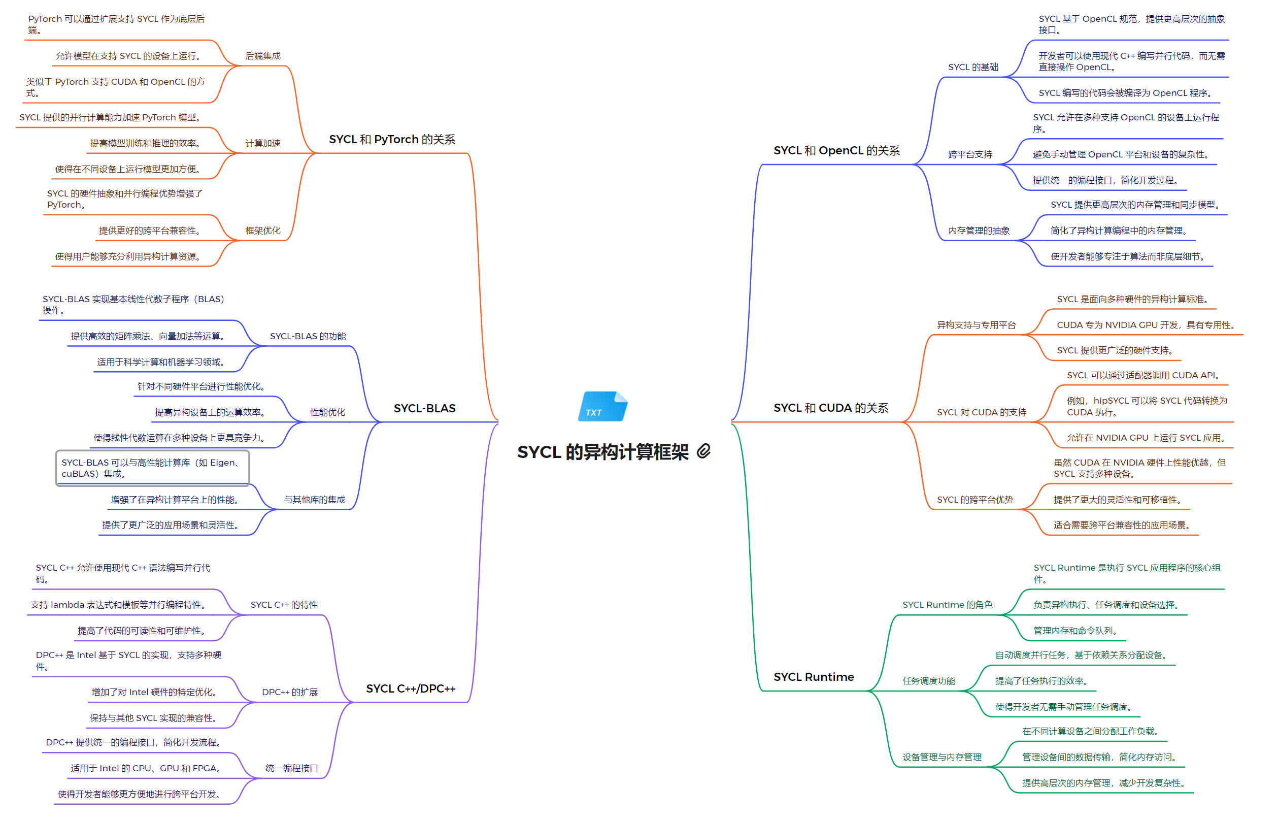
SYCL作为一个统一的高级抽象层,连接了多种底层计算技术,包括PyTorch、OpenCL和CUDA。在与PyTorch的集成方面,SYCL提供了计算加速和程序优化的能力,允许开发者利用SYCL的并行计算能力来增强PyTorch模型。对于OpenCL,SYCL简化了其使用复杂性,提供了更高级的抽象,同时保持了对OpenCL底层功能的访问能力。在CUDA方面,SYCL允许代码在NVIDIA GPU上运行,同时保持跨平台兼容性,为开发者提供了更大的灵活性。SYCL-BLAS作为一个重要组件,提供了高效的线性代数运算,支持各种硬件平台的优化。SYCL C++/DPC++扩展了C++标准,提供了更灵活的编程模型,特别适合Intel架构。SYCL Runtime作为核心组件,管理设备执行、内存同步、任务调度等关键功能,确保了跨平台的一致性和高效性。这种架构设计使SYCL能够在保持高性能的同时,提供了跨多种硬件平台的统一编程模型,大大简化了异构计算的开发复杂度,使开发者能够更容易地利用不同的加速器技术,同时保持代码的可移植性和效率。
系统软件层
该程序使用 SYCL 获取设备信息,并提取设备的名称、最大计算单元数和全局内存大小等信息,并将这些信息打印到控制台。
示例代码:
#include <CL/sycl.hpp>
#include <iostream>

int main() {
    try {
        // sycl::default_selector_v
        sycl::default_selector selector;
        sycl::queue queue(selector);

        // device
        sycl::device device = queue.get_device();

        std::cout << "Device Name: " << device.get_info<sycl::info::device::name>() << std::endl;
        std::cout << "Device Vendor: " << device.get_info<sycl::info::device::vendor>() << std::endl;
        std::cout << "Max Compute Units: " << device.get_info<sycl::info::device::max_compute_units>() << std::endl;
        std::cout << "Global Memory Size: " << device.get_info<sycl::info::device::global_mem_size>() / (1024 * 1024) << " MB" << std::endl;
    } catch (const sycl::exception& e) {
        std::cerr << "SYCL exception caught: " << e.what() << std::endl;
        return 1;
    }

    return 0;
}
结果:
Device Name: NVIDIA GeForce RTX 2080 Ti
Device Vendor: NVIDIA Corporation
Max Compute Units: 68
Global Memory Size: 11002 MB
运行时环境层
编程模型和语言层
SYCL是一个基于C++的高层次并行编程模型,旨在为异构计算提供更简单的开发体验。
1. SYCL 的核心编程特性
SYCL的编程模型主要包括以下关键特性:
- 单源编程 :SYCL允许开发者在同一个源文件中同时编写主机代码和设备代码。这种单源模型简化了代码管理,减少了代码的复杂性,使得编程过程更加直观。
- 队列与任务调度 :SYCL使用队列(queue)来管理内核的调度。开发者通过提交任务到队列来控制并行计算的执行。这种机制支持异步执行,使得主机可以在等待设备完成计算时进行其他任务。
- 内核(Kernel)函数 :SYCL内核是并行计算的核心,定义了在设备上执行的计算逻辑。内核函数使用sycl::handler进行调度,开发者可以通过指定的访问模式(如读、写)控制内存的访问。
__kernel void vectorAdd(__global const float* A, __global const float* B, __global float* C, int N) {
    int i = get_global_id(0);
    if (i < N) C[i] = A[i] + B[i];
}
上述示例展示了一个简单的内核,用于执行并行向量加法运算。
- 内存模型 :SYCL的内存模型允许开发者访问多种内存空间,包括全局内存、常量内存和私有内存。SYCL对内存的管理使得开发者能够更有效地利用硬件资源,并提升性能。
2. 算子编写示例:矩阵乘法
矩阵乘法是并行计算中常见的操作之一,下面展示如何在SYCL中实现并行矩阵乘法:
#include <CL/sycl.hpp>

void matrixMul(const float* A, const float* B, float* C, int N) {
    sycl::queue q;

    sycl::buffer<float, 1> bufA(A, sycl::range<1>(N * N));
    sycl::buffer<float, 1> bufB(B, sycl::range<1>(N * N));
    sycl::buffer<float, 1> bufC(C, sycl::range<1>(N * N));

    q.submit([&](sycl::handler& h) {
        auto accA = bufA.get_access<sycl::access::mode::read>(h);
        auto accB = bufB.get_access<sycl::access::mode::read>(h);
        auto accC = bufC.get_access<sycl::access::mode::write>(h);

        h.parallel_for(sycl::range<2>(N, N), [=](sycl::id<2> idx) {
            int row = idx[0];
            int col = idx[1];
            float result = 0.0f;
            for (int i = 0; i < N; ++i) {
                result += accA[row * N + i] * accB[i * N + col];
            }
            accC[row * N + col] = result;
        });
    }).wait(); // 同步等待计算完成
}
在这个示例中,内核函数负责并行计算矩阵的乘法,每个工作项处理结果矩阵中的一个元素。
3. 并行计算模型介绍
SYCL的并行计算模型灵活且强大,能够支持多种计算场景。以下是其主要概念:
- 工作项(Work-Item)与工作组(Work-Group) :SYCL将计算任务划分为工作项,每个工作项负责一部分计算。多个工作项组成工作组,工作组之间相互独立,而工作项可以共享局部内存,提高计算效率。
- 全局与局部内存 :SYCL允许工作项访问全局内存和局部内存。合理使用局部内存可以显著减少全局内存的访问次数,从而提升性能。
- 命令队列与同步 :主机通过命令队列提交计算任务,并可以使用事件机制来管理任务的执行和同步。这种机制使得开发者能够更好地控制任务的调度和资源利用。
4. SYCL与其他并行模型的对比
虽然SYCL与OpenCL和CUDA有相似之处,但它也有自己独特的优势:
- 跨平台性 :SYCL作为一个跨平台标准,可以在多种硬件架构上运行,支持开发者在不同设备上实现高效的并行计算。这使得SYCL在多样化的硬件环境中具有很强的适用性。
- 编程简易性 :SYCL提供了更高层次的抽象,允许开发者更专注于算法实现,而不必处理底层细节。这种简化的编程体验使得开发效率大大提高。
- 富的C++特性 :SYCL利用现代C++特性,如模板、Lambda表达式和类型推导,使得代码更加简洁和易于维护。
5. SYCL在AI开发中的应用
SYCL在AI开发中也展现出广泛的应用潜力,尤其是在以下场景中:
- 异构计算支持 :在需要同时利用多种硬件平台(如CPU和GPU)的AI应用中,SYCL的跨平台支持显得尤为重要。
- 边缘计算与嵌入式设备 :SYCL能够在资源有限的环境中提供强大的计算能力,适用于边缘计算和嵌入式AI设备。
- 深度学习框架的集成 :越来越多的深度学习框架开始支持SYCL,推动了在各种硬件平台上进行高效AI模型训练和推理的可能性。
6. 总结
SYCL作为现代异构计算的编程模型,为开发者提供了一种灵活且高效的方式来编写并行程序。其简化的编程体验和强大的跨平台能力,使得SYCL在AI技术栈中占据重要地位。理解SYCL的编程模型将帮助开发者在构建高效的AI系统时充分发挥硬件潜力,推动技术的进一步发展。
计算库层
portBLAS 使用 SYCL 实现 BLAS(基本线性代数例程),适用于现代异构计算平台。
参考仓库地址:portBLAS
blas::_gemm 通常是指 BLAS 库中的 gemm 函数,它执行矩阵-矩阵乘法。gemm 是 BLAS Level 3 例程中最核心的函数之一,它的全称是 "GEneral Matrix-Matrix multiplication"。
gemm 函数的基本操作是计算两个矩阵的乘积,并将结果加到第三个矩阵上,可以用以下数学公式表示:
C=α×A×B+β×C
其中:
- A 和 B 是输入矩阵。
- C 是输出矩阵,其内容在函数调用前可以是任意值。
- α 和 β 是标量倍数。
示例代码如下:
#include "portblas.hpp"
#include <sycl/sycl.hpp>

#include "util.hpp"

int main(int argc, char** argv) {
  /* Create a SYCL queue with the default device selector */
  sycl::queue q = sycl::queue(sycl::default_selector_v);

  /* Create a portBLAS sb_handle and get the policy handler */
  blas::SB_Handle sb_handle(q);

  /* Arguments of the Gemm operation.
   * Note: these matrix dimensions are too small to get a performance gain by
   * using portBLAS, but they are convenient for this sample */
  const size_t m = 7;
  const size_t k = 9;
  const size_t n = 5;
  const size_t lda = 12;
  const size_t ldb = 17;
  const size_t ldc = 10;
  const float alpha = 1.5;
  const float beta = 0.5;

  /* Create the matrices */
  std::vector<float> A = std::vector<float>(lda * k);
  std::vector<float> B = std::vector<float>(ldb * n);
  std::vector<float> C = std::vector<float>(ldc * n);

  /* Fill the matrices with random values */
  fill_matrix(A, m, k, lda);
  fill_matrix(B, k, n, ldb);
  fill_matrix(C, m, n, ldc);

  /* Print the matrices before the GEMM operation */
  std::cout << "A:\n";
  print_matrix(A, m, k, lda);
  std::cout << "---\nB:\n";
  print_matrix(B, k, n, ldb);
  std::cout << "---\nC (before):\n";
  print_matrix(C, m, n, ldc);

  /* Create the buffers */
  auto a_gpu = blas::make_sycl_iterator_buffer<float>(lda * k);
  auto b_gpu = blas::make_sycl_iterator_buffer<float>(ldb * n);
  auto c_gpu = blas::make_sycl_iterator_buffer<float>(ldc * n);

  /* Copy the matrices to the device
   * Note: this sample uses explicit copy operations, see the GEMV sample for
   * an alternative way
   */
  std::cout << "---\nCopying A, B and C to device\n";
  blas::helper::copy_to_device(sb_handle.get_queue(), A.data(), a_gpu, lda * k);
  blas::helper::copy_to_device(sb_handle.get_queue(), B.data(), b_gpu, ldb * n);
  blas::helper::copy_to_device(sb_handle.get_queue(), C.data(), c_gpu, ldc * n);

  /* Execute the GEMM operation */
  std::cout << "Executing C = " << alpha << "*A*B + " << beta << "*C\n";
  blas::_gemm(sb_handle, 'n', 'n', m, n, k, alpha, a_gpu, lda, b_gpu, ldb, beta,
              c_gpu, ldc);

  /* Copy the result to the host */
  std::cout << "Copying C to host\n";
  auto event = blas::helper::copy_to_host(sb_handle.get_queue(), c_gpu,
                                          C.data(), ldc * n);
  sb_handle.wait(event);

  /* Print the result after the GEMM operation */
  std::cout << "---\nC (after):" << std::endl;
  print_matrix(C, m, n, ldc);

  return 0;
}
结果:
A:
-1.438 9.5166 9.2763 9.7061 4.7123 -7.849 -5.247 -0.935 4.6360
-3.838 -9.125 -8.024 3.5507 9.6027 2.9939 8.8246 -3.819 1.4996
7.2394 3.6334 -6.483 5.1184 -0.098 -3.100 -3.855 2.2647 -2.312
-9.887 -4.862 -2.542 4.7151 -1.834 -6.717 6.3718 6.2206 -0.902
4.5156 -5.968 -1.436 4.9522 -2.603 9.3485 0.9153 8.6185 3.1563
-2.132 -7.835 -2.304 -3.719 -3.643 -7.861 4.0819 3.1938 -4.767
6.2794 9.6350 -1.894 -3.764 3.6267 -9.607 -3.615 -5.863 9.1741
---
B:
-5.155 8.9958 8.3243 -0.440 5.9613
0.6664 -6.633 -5.409 -9.602 6.2469
-4.575 4.5948 -7.293 1.4219 5.0536
-1.557 9.6612 2.7314 2.8409 9.9053
-5.624 1.0714 0.1577 -9.203 8.2468
-6.736 -8.187 -9.487 -1.367 2.2212
0.3280 8.0061 -7.627 -8.519 3.3489
8.2866 -6.657 -1.385 1.2509 0.0343
-1.143 8.3706 3.1169 -9.348 8.6974
---
C (before):
3.2586 0.6738 -0.649 -9.132 7.7019
-8.786 -5.771 0.5866 6.0604 -9.920
5.7516 -4.882 -1.464 -7.489 -1.981
-3.144 4.9594 3.2095 7.9944 8.8018
0.4556 9.3061 -6.114 -0.811 8.0797
5.1307 -4.322 7.5669 8.6118 6.9407
8.2092 -8.333 -4.818 2.2205 9.4932
---
Copying A, B and C to device
Executing C = 1.5*A*B + 0.5*C
Copying C to host
---
C (after):
-46.67 199.34 39.273 -128.2 360.91
-94.02 173.88 2.3888 -144.6 59.593
45.442 28.556 224.77 40.769 63.731
241.84 50.848 -30.16 77.259 -103.3
-12.70 32.391 -9.527 77.588 96.350
195.79 25.208 86.087 184.93 -274.5
-36.95 171.24 237.15 -285.7 194.97
blas::_gemv 是用于执行矩阵-向量乘法的例程。这里的 "gemv" 代表 "GEneral Matrix-Vector multiplication"。这个函数是 BLAS Level 2 例程的一部分,它提供了矩阵和向量之间的乘法操作。
示例代码如下:
#include "portblas.hpp"
#include <sycl/sycl.hpp>

#include "util.hpp"

int main(int argc, char** argv) {
  /* Create a SYCL queue with the default device selector */
  sycl::queue q = sycl::queue(sycl::default_selector_v);

  /* Create a portBLAS sb_handle and get the policy handler */
  blas::SB_Handle sb_handle(q);

  /* Arguments of the Gemm operation.
   * Note: these matrix dimensions are too small to get a performance gain by
   * using portBLAS, but they are convenient for this sample */
  const size_t m = 7;
  const size_t n = 7;
  const size_t lda = 12;
  const size_t incx = 2;
  const size_t incy = 3;
  const float alpha = 1.5;
  const float beta = 0.5;

  /* Create the matrix and vectors */
  const size_t lx = (n - 1) * incx + 1;
  const size_t ly = (m - 1) * incy + 1;
  std::vector<float> A = std::vector<float>(lda * n);
  std::vector<float> X = std::vector<float>(lx);
  std::vector<float> Y = std::vector<float>(ly);

  /* Fill the matrices with random values */
  fill_matrix(A, m, n, lda);
  fill_vector(X, n, incx);
  fill_vector(Y, m, incy);

  /* Print the matrices before the GEMV operation */
  std::cout << "A:\n";
  print_matrix(A, m, n, lda);
  std::cout << "---\nX:\n";
  print_vector(X, n, incx);
  std::cout << "---\nY (before):\n";
  print_vector(Y, m, incy);

  /* Execute the GEMV operation
   * Note: you can also use explicit copies, see the GEMM sample
   */
  std::cout << "---\nExecuting Y = " << alpha << "*A*X + " << beta << "*Y\n";
  {
    auto a_gpu = blas::make_sycl_iterator_buffer<float>(A, lda * n);
    auto x_gpu = blas::make_sycl_iterator_buffer<float>(X, lx);
    auto y_gpu = blas::make_sycl_iterator_buffer<float>(Y, ly);
    auto event = blas::_gemv(sb_handle, 'n', m, n, alpha, a_gpu, lda, x_gpu,
                             incx, beta, y_gpu, incy);
  }

  /* Print the result after the GEMM operation */
  std::cout << "---\nY (after):" << std::endl;
  print_vector(Y, m, incy);

  return 0;
}
结果:
A:
3.6917 7.9525 0.9778 1.6808 -4.840 -3.500 -5.867
1.6618 -4.460 5.0066 8.7876 1.7519 5.5783 -7.085
-5.231 0.6601 0.5053 -1.237 -5.133 -7.862 -4.636
7.9965 -2.646 5.6696 1.9292 -1.571 3.1671 -2.653
-5.239 3.9521 -1.618 -4.856 4.8694 5.0238 3.2869
-0.183 0.5850 -1.778 0.6833 -7.747 0.8794 9.6463
0.8742 -9.219 -8.838 -4.268 2.2112 3.4617 -8.035
---
X:
5.5933
-2.949
8.8669
6.9684
-1.255
-7.447
-2.448
---
Y (before):
4.0870
-9.189
-8.224
-1.195
-7.723
-6.854
-1.389
---
Executing Y = 1.5*A*X + 0.5*Y
---
Y (after):
98.187
147.93
57.397
151.09
-214.9
-54.74
-128.0
框架模型层
Triton (NVIDIA)
Triton 是一个创新的开源项目,旨在简化 GPU 编程并提高计算性能。它提供了一种高级抽象,使开发者能够更容易地编写高效的 GPU 内核,而无需深入了解底层硬件细节。Triton 的设计理念是在保持高性能的同时,提供更好的可读性和可维护性。
Triton 引入了几个关键概念:
-
Triton DSL(领域特定语言):Triton 提供了一种特定于 GPU 编程的语言,它是 Python 的一个子集,增加了一些特定于并行计算的原语。
-
自动调优:Triton 能够自动选择最佳的执行参数,如线程块大小和内存访问模式。
-
多维张量操作: Triton 原生支持多维张量操作,使得复杂的数学运算变得简单。
-
动态形状支持:与传统 CUDA 编程不同,Triton 支持动态形状的输入,增加了代码的灵活性。
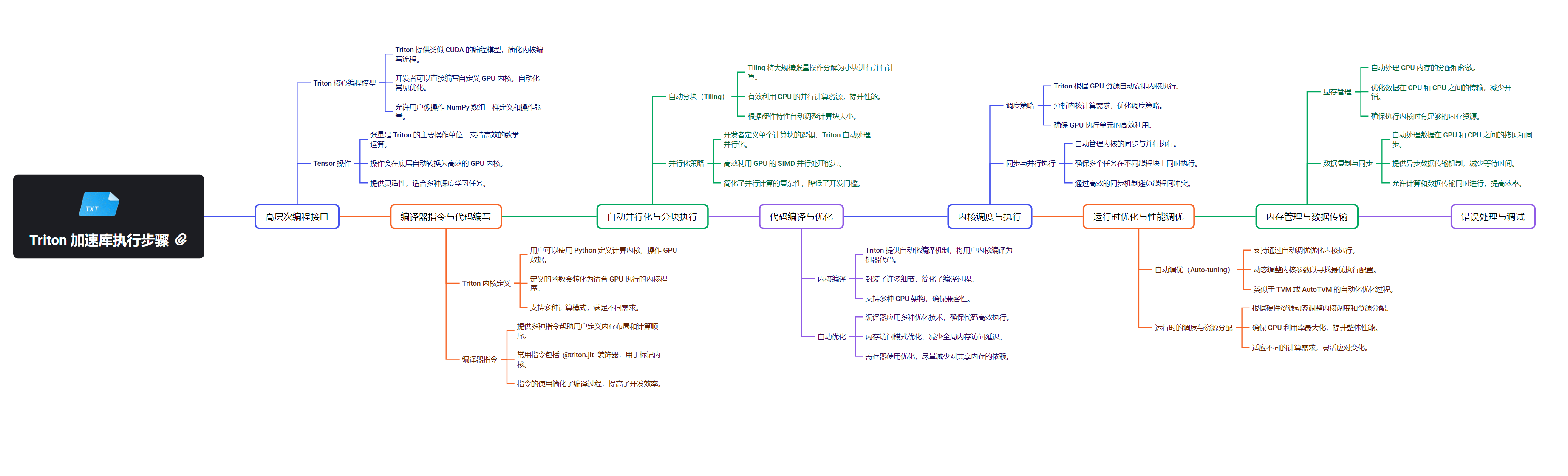
Triton 的工作原理
Triton 的工作原理可以分为以下几个关键步骤:
- 代码分析:Triton 编译器分析用 Triton DSL 编写的代码。
- 中间表示生成:将代码转换为 MLIR(Multi-Level Intermediate Representation)。
- 优化:在 MLIR 层面进行各种优化。
- 代码生成:将优化后的 MLIR 转换为目标硬件的机器代码(如 PTX 或 AMDGPU ISA)。
- 运行时执行:使用相应的 GPU API 加载和执行生成的代码。
Triton 的编译流程
Triton 的编译流程是其核心优势之一,包括以下主要阶段:
-
Triton DSL → MLIR
- 解析 Triton DSL 代码
- 生成初始的 MLIR 表示
-
MLIR 优化
- 执行特定于 Triton 的优化pass
- 应用通用的 MLIR 优化
-
MLIR → LLVM IR
- 将优化后的 MLIR 转换为 LLVM IR
-
LLVM IR → 目标代码
- 使用 LLVM 后端生成目标特定的机器代码(如 PTX)
-
JIT 编译
- 在运行时即时编译生成的代码
这个流程允许 Triton 在保持高级抽象的同时,生成高度优化的机器代码。
与 GPU Runtime 和 API 的对接
Triton 通过多层抽象与不同的 GPU 平台进行交互:
- CUDA Driver API
- 使用低级 API 如
cuModuleLoad和cuLaunchKernel加载和执行 PTX 代码。
- CUDA Runtime API
- 利用更高级的 API 如
cudaLaunchKernel简化内核启动过程。
- ROCm 和 HIP API
- 为 AMD GPU 提供支持,使用 HIP API 进行交互。
- 具体实现细节
- 代码生成:生成适合目标平台的代码(PTX 或 AMDGPU ISA)。
- 运行时集成:创建封装底层 API 调用的 GPU Driver 对象。
- 内核加载与启动:使用相应的 API 加载编译好的 GPU 代码并启动内核。
- 结果获取与错误处理:同步执行结果,处理可能的错误。
Triton 的抽象层
Triton 提供了多个抽象层,以简化跨平台 GPU 编程:
设备抽象
- 定义通用的 Device 接口,隐藏不同 GPU 架构的细节。
内存管理抽象
- 提供统一的内存分配和数据传输接口。
内核启动抽象
- 简化不同平台上的内核配置和启动过程。
编程模型抽象
- 提供统一的编程模型,使开发者能够编写可移植的代码。
Triton 与 PyTorch 的集成
Triton 可以与 PyTorch 无缝集成,为深度学习模型提供性能优化:
自定义 CUDA 内核
- 使用 Triton 编写高效的自定义操作,集成到 PyTorch 模型中。
性能关键操作的优化
- 针对特定的计算密集型操作,如矩阵乘法,使用 Triton 实现高性能版本。
Triton 的优势与局限性
优势
- 简化 GPU 编程,提高开发效率。
- 自动优化,减少手动调优的需求。
- 良好的可移植性,支持多种 GPU 架构。
- 与 PyTorch 等深度学习框架的无缝集成。
局限性
- 学习曲线可能较陡,特别是对于不熟悉 GPU 编程的开发者。
- 在某些极端情况下,手动优化的 CUDA 代码可能仍然更快。
- 生态系统相对较新,社区支持和工具链还在发展中。
技术栈架构
1. 系统软件层
- NVIDIA GPU 驱动:为 GPU 提供基本的系统级支持。
- CUDA Driver API:低级 API,提供对 GPU 的直接控制。
- 允许直接管理设备、内存分配和程序执行。
- 适用于需要细粒度控制的高级应用。
- 提供与 NVIDIA GPU 硬件交互的底层接口。
2. 运行时环境层
- CUDA Runtime API:高级 API,简化了 GPU 编程,自动管理许多底层细节。
- 提供更高级的抽象,简化了 GPU 的使用。
- 自动处理上下文管理和程序加载等任务。
- 更适合一般开发者使用,提供了更好的易用性。
3. 编程模型和语言层
- Triton DSL (领域特定语言):扩展了 Python,允许开发者编写在 GPU 上运行的并行程序。
- 允许在 CPU 和 GPU 上混合编程。
- 使用 Triton 特定语法定义 GPU 函数。
- 通过方言(Dialect)提供优化的操作和功能。
4. 计算库层
- Triton 实现的算子库:提供高性能的计算内核,专门针对各种深度学习操作进行优化。
- 针对特定操作的高效实现,如矩阵运算。
5. 框架模型层
- PyTorch:支持动态计算图的深度学习框架,通过
torch.cuda模块提供 CUDA 功能。- 自动管理 GPU 内存,支持 GPU 和 CPU 之间的数据转移。
- TensorFlow:支持静态和动态计算图的深度学习框架。
- 通过 XLA 编译器优化 GPU 代码执行,提供高级 API 来简化 CUDA API 的使用。
关系解析
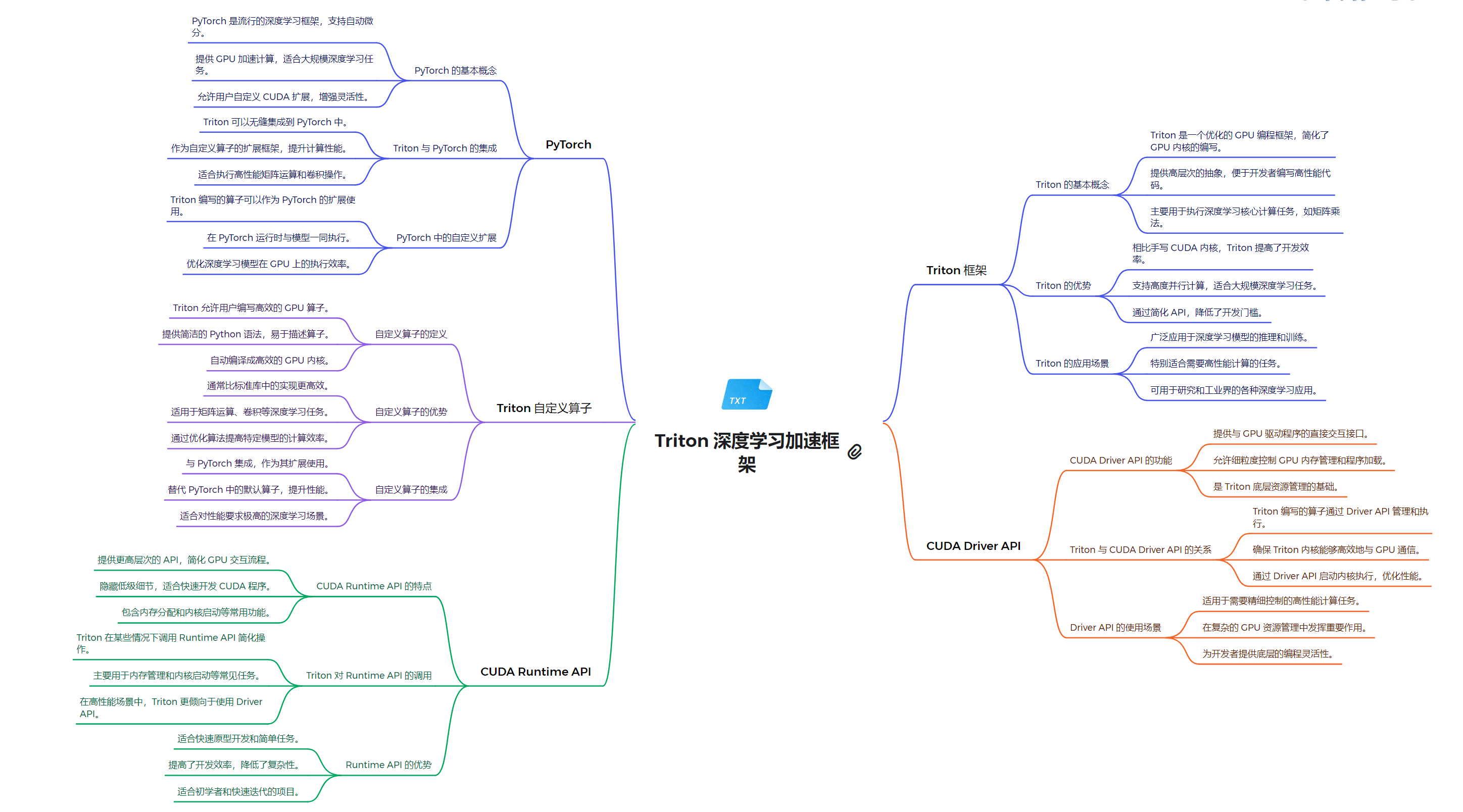 本图展示了Triton深度学习加速框架的核心组成和技术关系。Triton作为中心,与PyTorch、CUDA Runtime API和CUDA Driver API形成了紧密的技术生态。在PyTorch方面,Triton通过自定义算子、JIT编译和GPU内核融合等技术,显著提升了深度学习模型的性能。Triton自定义算子部分详细阐述了其如何优化内存访问、自动并行化以及与PyTorch的无缝集成。在底层,Triton通过CUDA Runtime API实现了高效的GPU编程,包括内存管理、设备操作和kernel启动等功能。同时,Triton还利用CUDA Driver API进行更底层的硬件控制和优化,如直接管理GPU上下文、内存分配和设备属性查询等。这种多层次的架构设计使Triton能够在保持高度灵活性的同时,提供卓越的性能优化,特别是在复杂的深度学习工作负载中。通过整合这些技术,Triton为开发者提供了一个强大的工具,能够充分利用GPU的计算能力,同时简化了高性能深度学习应用的开发过程。
系统软件层
Triton 通过使用 CUDA Driver API 与底层 GPU 进行交互。具体流程如下:
- Triton 生成的代码将被编译为 PTX(Parallel Thread Execution)代码,用于 NVIDIA GPU。
- 通过 CUDA Driver API(例如
cuModuleLoad,cuLaunchKernel等)来加载和执行这些 PTX 代码。
使用 CUDA Driver API 来进行简单的 GPU 内存分配和向量加法计算,示例代码如下:
PTX 文件:
__global__ void vecAdd(float *A, float *B, float *C, int N) {
    int i = blockIdx.x * blockDim.x + threadIdx.x;
    if (i < N) {
        C[i] = A[i] + B[i];
    }
}
程序:
#include <cuda.h>
#include <stdio.h>
#include <stdlib.h>

#define CHECK_CUDA_RESULT(res, msg) \
    if (res != CUDA_SUCCESS) { \
        printf("Error: %s, CUDA result: %d\n", msg, res); \
        return -1; \
    }

int main() {
    CUdevice cuDevice;
    CUcontext cuContext;
    CUmodule cuModule;
    CUfunction cuFunction;
    CUresult res;

    int N = 512;
    size_t size = N * sizeof(float);

    // Initialize the CUDA Driver API
    res = cuInit(0);
    CHECK_CUDA_RESULT(res, "cuInit failed");

    // Get the device and create a context
    res = cuDeviceGet(&cuDevice, 0);
    CHECK_CUDA_RESULT(res, "cuDeviceGet failed");

    res = cuCtxCreate(&cuContext, 0, cuDevice);
    CHECK_CUDA_RESULT(res, "cuCtxCreate failed");

    // Allocate device memory
    CUdeviceptr d_A, d_B, d_C;
    res = cuMemAlloc(&d_A, size);
    CHECK_CUDA_RESULT(res, "cuMemAlloc for A failed");

    res = cuMemAlloc(&d_B, size);
    CHECK_CUDA_RESULT(res, "cuMemAlloc for B failed");

    res = cuMemAlloc(&d_C, size);
    CHECK_CUDA_RESULT(res, "cuMemAlloc for C failed");

    // Initialize host arrays and copy data to device
    float *h_A = (float *)malloc(size);
    float *h_B = (float *)malloc(size);
    float *h_C = (float *)malloc(size);

    for (int i = 0; i < N; ++i) {
        h_A[i] = i; // Example values
        h_B[i] = i; // Example values
    }

    // Copy data from host to device
    res = cuMemcpyHtoD(d_A, h_A, size);
    CHECK_CUDA_RESULT(res, "cuMemcpyHtoD for A failed");

    res = cuMemcpyHtoD(d_B, h_B, size);
    CHECK_CUDA_RESULT(res, "cuMemcpyHtoD for B failed");

    // Load the compiled PTX module and get the kernel function
    const char *kernel_file = "add.ptx"; // Precompiled PTX file
    res = cuModuleLoad(&cuModule, kernel_file);
    CHECK_CUDA_RESULT(res, "cuModuleLoad failed");

    res = cuModuleGetFunction(&cuFunction, cuModule, "_Z6vecAddPfS_S_i"); // Adjust if needed
    CHECK_CUDA_RESULT(res, "cuModuleGetFunction failed");

    // Set kernel parameters and launch the kernel
    void *args[] = { &d_A, &d_B, &d_C, &N };
    res = cuLaunchKernel(
        cuFunction,        // Kernel to launch
        (N + 255) / 256, 1, 1,     // Grid dimensions
        256, 1, 1,         // Block dimensions
        0,                 // Shared memory size
        0,                 // Stream
        args,              // Kernel arguments
        NULL               // Extra options
    );
    CHECK_CUDA_RESULT(res, "cuLaunchKernel failed");

    // Synchronize to ensure kernel execution is complete
    res = cuCtxSynchronize();
    CHECK_CUDA_RESULT(res, "cuCtxSynchronize failed");

    // Copy the result back to the host
    res = cuMemcpyDtoH(h_C, d_C, size);
    CHECK_CUDA_RESULT(res, "cuMemcpyDtoH for C failed");

    // Print the results
    for (int i = 0; i < N; ++i) {
        printf("%f + %f = %f\n", h_A[i], h_B[i], h_C[i]);
    }

    // Free device memory and destroy the context
    cuMemFree(d_A);
    cuMemFree(d_B);
    cuMemFree(d_C);
    cuCtxDestroy(cuContext);

    // Free host memory
    free(h_A);
    free(h_B);
    free(h_C);

    return 0;
}
结果:
0.000000 + 0.000000 = 0.000000
1.000000 + 1.000000 = 2.000000
2.000000 + 2.000000 = 4.000000
3.000000 + 3.000000 = 6.000000
4.000000 + 4.000000 = 8.000000
5.000000 + 5.000000 = 10.000000
...
510.000000 + 510.000000 = 1020.000000
511.000000 + 511.000000 = 1022.000000
运行时环境层
Triton 的设计使得它能够灵活地与 GPU 进行交互,涉及多个层次的抽象和转换。
除了 CUDA Driver API,Triton 还可以利用 CUDA Runtime API,这是建立在 Driver API 之上的更高级别接口,常见的操作包括:
- 使用
cudaLaunchKernel来启动内核。 - 为 AMD GPU 提供支持,使用 ROCm 与 HIP API 进行交互。
运行时环境层构建在系统软件层之上,负责为 Triton 生成的内核代码提供执行和优化的运行环境。这个层次主要关注高效的硬件资源利用、执行调度和运行时的动态优化。
1. CUDA Runtime API
- 功能 :CUDA Runtime API 提供了高层次的编程接口,简化了与 GPU 的交互。开发者通过它可以实现更高级别的内存管理、数据传输和内核调度。
- 与 Triton 的关系 :Triton 通过 CUDA Runtime API 管理内存分配、数据传输以及内核执行的生命周期。例如,Triton 的内核在 GPU 上执行时,Runtime API 管理着内核的调度以及执行顺序。
2. Kernel Fusion (内核融合)
- 作用 :Triton 运行时具有内核融合的能力,能够将多个计算内核融合成一个内核执行,减少数据传输的开销和启动内核的延迟。这对 AI 模型的性能优化至关重要,尤其是在大规模矩阵运算和卷积操作中。
- 原理 :通过合并多个计算任务为一个大的并行执行任务,Triton 可以最大化利用 GPU 的计算单元和内存带宽,减少上下文切换的开销。
3. 动态并行性 (Dynamic Parallelism)
- 作用 :Triton 依赖 CUDA 的动态并行性特性,使得内核能够在 GPU 上直接启动其他内核,减少了 CPU 与 GPU 之间的通信开销。这使得在复杂的 AI 模型中,可以充分利用 GPU 的计算能力,优化多阶段计算任务。
- 应用场景 :在深度学习中,复杂的前向传播和反向传播过程都可以通过动态并行性高效地在 GPU 上完成。
4. 内存管理与优化
- 统一内存(Unified Memory) :CUDA Runtime 提供了统一内存的支持,Triton 可以使用统一内存模型自动在 CPU 和 GPU 之间进行数据管理,减少了开发者手动进行内存复制的复杂性。
- 共享内存与寄存器 :Triton 的代码生成器会针对每个 CUDA 内核最大化利用 GPU 的共享内存和寄存器资源,以减少全局内存的访问延迟,提高并行任务的执行效率。
5. 异步执行与流(Streams)
- 功能 :Triton 运行时支持异步执行,通过 CUDA Streams 来管理多个任务的并发执行。通过将不同的内核任务放置在不同的流中,Triton 能够实现高效的任务并行,减少 GPU 闲置时间。
- 优势 :异步执行模型能够避免数据传输和内核执行之间的等待时间,从而提高整体计算性能。
示例代码如下:
#include <cuda_runtime.h>
#include <stdio.h>

__global__ void vecAdd(float *A, float *B, float *C, int N) {
    int i = blockIdx.x * blockDim.x + threadIdx.x;
    if (i < N) {
        C[i] = A[i] + B[i];
    }
}

int main() {
    int N = 512;
    size_t size = N * sizeof(float);

    // Allocate host memory
    float *h_A = (float *)malloc(size);
    float *h_B = (float *)malloc(size);
    float *h_C = (float *)malloc(size);

    // Initialize host arrays
    for (int i = 0; i < N; i++) {
        h_A[i] = i;
        h_B[i] = i * 2;
    }

    // Allocate device memory
    float *d_A, *d_B, *d_C;
    cudaMalloc((void **)&d_A, size);
    cudaMalloc((void **)&d_B, size);
    cudaMalloc((void **)&d_C, size);

    // Copy data from host to device
    cudaMemcpy(d_A, h_A, size, cudaMemcpyHostToDevice);
    cudaMemcpy(d_B, h_B, size, cudaMemcpyHostToDevice);

    // Set kernel launch configuration
    int threadsPerBlock = 256;
    int blocksPerGrid = (N + threadsPerBlock - 1) / threadsPerBlock;

    // Launch the kernel
    vecAdd<<<blocksPerGrid, threadsPerBlock>>>(d_A, d_B, d_C, N);

    // Copy result back to host
    cudaMemcpy(h_C, d_C, size, cudaMemcpyDeviceToHost);

    // Print out part of the result to verify it
    printf("Result of vector addition (first 10 elements):\n");
    for (int i = 0; i < 10; i++) {
        printf("C[%d] = %f\n", i, h_C[i]);
    }

    // Free device and host memory
    cudaFree(d_A);
    cudaFree(d_B);
    cudaFree(d_C);
    free(h_A);
    free(h_B);
    free(h_C);

    return 0;
}
结果:
Result of vector addition (first 10 elements):
C[0] = 0.000000
C[1] = 3.000000
C[2] = 6.000000
C[3] = 9.000000
C[4] = 12.000000
C[5] = 15.000000
C[6] = 18.000000
C[7] = 21.000000
C[8] = 24.000000
C[9] = 27.000000
这个示例展示了如何通过 CUDA Runtime API 管理内存、数据传输和内核执行。
- 内存管理 :使用
cudaMalloc()和cudaMemcpy()管理设备内存和主机到设备的数据传输。 - 内核执行 :通过
<<<blocksPerGrid, threadsPerBlock>>>的方式启动内核。 - 数据传输和同步 :使用
cudaMemcpy()将计算结果从设备传回主机,并通过cudaFree()释放内存。
编程模型和语言层
Triton 语言是为高性能计算而设计的领域特定语言 (DSL),由OpenAI开发,Triton允许用户使用简洁的Python接口编写自定义的GPU内核,同时具备高性能优化的能力。
1. Triton 的核心编程特性
Triton的编程模型主要包括以下关键特性:
- 简洁的内核编写 :Triton允许开发者使用类似Python的语法来编写GPU内核。通过高层次的抽象,开发者可以更专注于算法实现,而不必深入底层CUDA的复杂性。
- 自动优化 :Triton自动处理内核的优化过程,包括内存访问模式、线程布局等。开发者只需关注算法逻辑,Triton会在后台生成高效的机器代码。
- 灵活的调度策略 :Triton提供了多种调度策略,以适应不同的计算需求。开发者可以根据具体场景选择最适合的调度方式,从而提高性能。
2. 算子编写示例:矩阵加法
以下是一个使用Triton实现向量加法的示例:
import triton
import triton.language as tl

@triton.jit
def vector_add(A, B, C, n):
    pid = tl.program_id(0)
    start = pid * BLOCK_SIZE
    end = min(start + BLOCK_SIZE, n)
    for i in range(start, end):
        C[i] = A[i] + B[i]

def run_vector_add(A, B, C, n):
    vector_add[(n + BLOCK_SIZE - 1) // BLOCK_SIZE](A, B, C, n)
在此示例中,vector_add函数定义了在GPU上执行的内核逻辑,run_vector_add函数则负责调度内核执行。
3. 并行计算模型介绍
Triton的并行计算模型设计为高效支持GPU的异构计算,主要概念包括:
- 程序ID和块 :Triton通过program_id函数管理计算任务的划分。每个程序ID对应一个计算块,开发者可以控制每个块处理的数据范围。
- 共享内存与全局内存 :Triton允许内核使用共享内存以提升性能,同时也支持全局内存的访问。合理配置内存使用可以显著提升内核的计算效率。
- 异步执行与同步 :Triton支持异步内核执行,允许主机在等待GPU计算完成时进行其他任务。这种机制提高了资源利用率和执行效率。
4. Triton与其他并行模型的对比
虽然Triton在某些方面与CUDA和OpenCL类似,但它在高层抽象和用户体验上有其独特之处:
- 易用性 :Triton以Python为基础,提供了更为简洁和直观的编程体验。相比CUDA,Triton的学习曲线较为平缓,适合广泛的用户群体。
- 自动优化 :Triton的自动优化机制显著减少了开发者的手动调优工作,使得高性能内核的编写变得更加简单。
- 高层次抽象 :Triton通过高层次的编程模型降低了对底层硬件细节的关注,使得开发者可以快速实现和测试新的算法。
5. Triton在AI开发中的应用
Triton在AI开发中展现了广泛的应用潜力,特别是在以下场景中:
- 深度学习框架的集成 :Triton可以与现有的深度学习框架(如PyTorch)无缝集成,帮助开发者快速实现自定义算子,提高模型性能。
- 快速原型开发 :由于其易用性,Triton特别适合快速原型开发,研究者可以迅速测试新的算法和想法。
- 高性能计算需求 :在需要高性能计算的深度学习任务中,Triton的优化能力使其成为理想选择,尤其是在处理大规模数据时。
6. 总结
Triton作为一个新兴的深度学习编程框架,为GPU计算提供了一种高效且易于使用的编程方式。通过简化内核编写和自动优化,Triton在AI技术栈中占据了重要地位。理解Triton的编程模型将帮助开发者在构建高效的深度学习系统时充分发挥GPU的潜力,推动技术的进一步发展。
计算库层
Triton 提供了高性能的计算库,开发者可以利用这些库进行高效操作。例如,标准的Add(向量加法)、 GEMM(矩阵乘法)等操作可以使用 Triton 的编程模型实现,利用自定义内存访问模式和自动调优功能获得更佳性能。
参考仓库地址:triton
向量加法的实现示例代码如下:
"""
Vector Addition
===============

In this tutorial, you will write a simple vector addition using Triton.

In doing so, you will learn about:

* The basic programming model of Triton.

* The `triton.jit` decorator, which is used to define Triton kernels.

* The best practices for validating and benchmarking your custom ops against native reference implementations.

"""

# %%
# Compute Kernel
# --------------

import torch

import triton
import triton.language as tl

@triton.jit
def add_kernel(x_ptr,  # *Pointer* to first input vector.
               y_ptr,  # *Pointer* to second input vector.
               output_ptr,  # *Pointer* to output vector.
               n_elements,  # Size of the vector.
               BLOCK_SIZE: tl.constexpr,  # Number of elements each program should process.
               # NOTE: `constexpr` so it can be used as a shape value.
               ):
    # There are multiple 'programs' processing different data. We identify which program
    # we are here:
    pid = tl.program_id(axis=0)  # We use a 1D launch grid so axis is 0.
    # This program will process inputs that are offset from the initial data.
    # For instance, if you had a vector of length 256 and block_size of 64, the programs
    # would each access the elements [0:64, 64:128, 128:192, 192:256].
    # Note that offsets is a list of pointers:
    block_start = pid * BLOCK_SIZE
    offsets = block_start + tl.arange(0, BLOCK_SIZE)
    # Create a mask to guard memory operations against out-of-bounds accesses.
    mask = offsets < n_elements
    # Load x and y from DRAM, masking out any extra elements in case the input is not a
    # multiple of the block size.
    x = tl.load(x_ptr + offsets, mask=mask)
    y = tl.load(y_ptr + offsets, mask=mask)
    output = x + y
    # Write x + y back to DRAM.
    tl.store(output_ptr + offsets, output, mask=mask)

# %%
# Let's also declare a helper function to (1) allocate the `z` tensor
# and (2) enqueue the above kernel with appropriate grid/block sizes:

def add(x: torch.Tensor, y: torch.Tensor):
    # We need to preallocate the output.
    output = torch.empty_like(x)
    assert x.is_cuda and y.is_cuda and output.is_cuda
    n_elements = output.numel()
    # The SPMD launch grid denotes the number of kernel instances that run in parallel.
    # It is analogous to CUDA launch grids. It can be either Tuple[int], or Callable(metaparameters) -> Tuple[int].
    # In this case, we use a 1D grid where the size is the number of blocks:
    grid = lambda meta: (triton.cdiv(n_elements, meta['BLOCK_SIZE']), )
    # NOTE:
    #  - Each torch.tensor object is implicitly converted into a pointer to its first element.
    #  - `triton.jit`'ed functions can be indexed with a launch grid to obtain a callable GPU kernel.
    #  - Don't forget to pass meta-parameters as keywords arguments.
    add_kernel[grid](x, y, output, n_elements, BLOCK_SIZE=1024)
    # We return a handle to z but, since `torch.cuda.synchronize()` hasn't been called, the kernel is still
    # running asynchronously at this point.
    return output

# %%
# We can now use the above function to compute the element-wise sum of two `torch.tensor` objects and test its correctness:

torch.manual_seed(0)
size = 98432
x = torch.rand(size, device='cuda')
y = torch.rand(size, device='cuda')
output_torch = x + y
output_triton = add(x, y)
print(output_torch)
print(output_triton)
print(f'The maximum difference between torch and triton is '
      f'{torch.max(torch.abs(output_torch - output_triton))}')

# %%
# Seems like we're good to go!

# %%
# Benchmark
# ---------
#
# We can now benchmark our custom op on vectors of increasing sizes to get a sense of how it does relative to PyTorch.
# To make things easier, Triton has a set of built-in utilities that allow us to concisely plot the performance of our custom ops.
# for different problem sizes.


@triton.testing.perf_report(
    triton.testing.Benchmark(
        x_names=['size'],  # Argument names to use as an x-axis for the plot.
        x_vals=[2**i for i in range(12, 28, 1)],  # Different possible values for `x_name`.
        x_log=True,  # x axis is logarithmic.
        line_arg='provider',  # Argument name whose value corresponds to a different line in the plot.
        line_vals=['triton', 'torch'],  # Possible values for `line_arg`.
        line_names=['Triton', 'Torch'],  # Label name for the lines.
        styles=[('blue', '-'), ('green', '-')],  # Line styles.
        ylabel='GB/s',  # Label name for the y-axis.
        plot_name='vector-add-performance',  # Name for the plot. Used also as a file name for saving the plot.
        args={},  # Values for function arguments not in `x_names` and `y_name`.
    ))
def benchmark(size, provider):
    x = torch.rand(size, device='cuda', dtype=torch.float32)
    y = torch.rand(size, device='cuda', dtype=torch.float32)
    quantiles = [0.5, 0.2, 0.8]
    if provider == 'torch':
        ms, min_ms, max_ms = triton.testing.do_bench(lambda: x + y, quantiles=quantiles)
    if provider == 'triton':
        ms, min_ms, max_ms = triton.testing.do_bench(lambda: add(x, y), quantiles=quantiles)
    gbps = lambda ms: 3 * x.numel() * x.element_size() / ms * 1e-6
    return gbps(ms), gbps(max_ms), gbps(min_ms)

# %%
# We can now run the decorated function above. Pass `print_data=True` to see the performance number, `show_plots=True` to plot them, and/or
# `save_path='/path/to/results/' to save them to disk along with raw CSV data:
benchmark.run(print_data=True, show_plots=True, save_path="output")
结果:
tensor([1.3713, 1.3076, 0.4940,  ..., 0.6724, 1.2141, 0.9733], device='cuda:0')
tensor([1.3713, 1.3076, 0.4940,  ..., 0.6724, 1.2141, 0.9733], device='cuda:0')
The maximum difference between torch and triton is 0.0
vector-add-performance:
           size      Triton       Torch
0        4096.0   12.000000   12.000000
1        8192.0   24.000000   24.000000
2       16384.0   44.846717   44.521738
3       32768.0   76.800002   76.800002
4       65536.0  148.048195  151.703707
5      131072.0  219.428568  222.407245
6      262144.0  341.333321  365.442364
7      524288.0  433.534740  409.600010
8     1048576.0  506.069512  491.520012
9     2097152.0  534.260858  546.133325
10    4194304.0  564.965515  564.965515
11    8388608.0  606.522314  603.092009
12   16777216.0  620.214515  611.949793
13   33554432.0  632.084809  627.310727
14   67108864.0  635.243943  642.034476
15  134217728.0  638.078725  633.441130
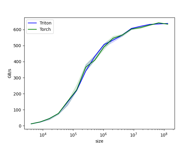 下面将实现一个融合的 softmax 操作,该操作在处理特定类型的矩阵时,性能显著优于 PyTorch 的原生实现。具体而言,当矩阵的行可以适应 GPU 的 SRAM 时,融合内核可以减少内存访问并提高计算效率。通过这个例子,我们将学习内核融合的好处以及 Triton 中的归约操作。
融合的 softmax实现示例代码如下:
"""
Fused Softmax
=============

In this tutorial, you will write a fused softmax operation that is significantly faster
than PyTorch's native op for a particular class of matrices: those whose rows can fit in
the GPU's SRAM.

In doing so, you will learn about:

* The benefits of kernel fusion for bandwidth-bound operations.

* Reduction operators in Triton.

"""

# %%
# Motivations
# -----------
#
# Custom GPU kernels for elementwise additions are educationally valuable but won't get you very far in practice.
# Let us consider instead the case of a simple (numerically stabilized) softmax operation:

import torch

import triton
import triton.language as tl
from triton.runtime import driver

def is_hip():
    return triton.runtime.driver.active.get_current_target().backend == "hip"

def is_cdna():
    return is_hip() and triton.runtime.driver.active.get_current_target().arch in ('gfx940', 'gfx941', 'gfx942',
                                                                                   'gfx90a', 'gfx908')

def naive_softmax(x):
    """Compute row-wise softmax of X using native pytorch

    We subtract the maximum element in order to avoid overflows. Softmax is invariant to
    this shift.
    """
    # read  MN elements ; write M  elements
    x_max = x.max(dim=1)[0]
    # read MN + M elements ; write MN elements
    z = x - x_max[:, None]
    # read  MN elements ; write MN elements
    numerator = torch.exp(z)
    # read  MN elements ; write M  elements
    denominator = numerator.sum(dim=1)
    # read MN + M elements ; write MN elements
    ret = numerator / denominator[:, None]
    # in total: read 5MN + 2M elements ; wrote 3MN + 2M elements
    return ret

# %%
# When implemented naively in PyTorch, computing :code:`y = naive_softmax(x)` for :math:`x \in R^{M \times N}`
# requires reading :math:`5MN + 2M` elements from DRAM and writing back :math:`3MN + 2M` elements.
# This is obviously wasteful; we'd prefer to have a custom "fused" kernel that only reads
# X once and does all the necessary computations on-chip.
# Doing so would require reading and writing back only :math:`MN` bytes, so we could
# expect a theoretical speed-up of ~4x (i.e., :math:`(8MN + 4M) / 2MN`).
# The `torch.jit.script` flags aims to perform this kind of "kernel fusion" automatically
# but, as we will see later, it is still far from ideal.

# %%
# Compute Kernel
# --------------
#
# Our softmax kernel works as follows: each program loads a set of rows of the input matrix X strided by number of programs,
# normalizes it and writes back the result to the output Y.
#
# Note that one important limitation of Triton is that each block must have a
# power-of-two number of elements, so we need to internally "pad" each row and guard the
# memory operations properly if we want to handle any possible input shapes:


@triton.jit
def softmax_kernel(output_ptr, input_ptr, input_row_stride, output_row_stride, n_rows, n_cols, BLOCK_SIZE: tl.constexpr,
                   num_stages: tl.constexpr):
    # starting row of the program
    row_start = tl.program_id(0)
    row_step = tl.num_programs(0)
    for row_idx in tl.range(row_start, n_rows, row_step, num_stages=num_stages):
        # The stride represents how much we need to increase the pointer to advance 1 row
        row_start_ptr = input_ptr + row_idx * input_row_stride
        # The block size is the next power of two greater than n_cols, so we can fit each
        # row in a single block
        col_offsets = tl.arange(0, BLOCK_SIZE)
        input_ptrs = row_start_ptr + col_offsets
        # Load the row into SRAM, using a mask since BLOCK_SIZE may be > than n_cols
        mask = col_offsets < n_cols
        row = tl.load(input_ptrs, mask=mask, other=-float('inf'))
        # Subtract maximum for numerical stability
        row_minus_max = row - tl.max(row, axis=0)
        # Note that exponentiation in Triton is fast but approximate (i.e., think __expf in CUDA)
        numerator = tl.exp(row_minus_max)
        denominator = tl.sum(numerator, axis=0)
        softmax_output = numerator / denominator
        # Write back output to DRAM
        output_row_start_ptr = output_ptr + row_idx * output_row_stride
        output_ptrs = output_row_start_ptr + col_offsets
        tl.store(output_ptrs, softmax_output, mask=mask)

# %%
# We can create a helper function that enqueues the kernel and its (meta-)arguments for any given input tensor.

device = torch.cuda.current_device()
properties = driver.active.utils.get_device_properties(device)
NUM_SM = properties["multiprocessor_count"]
NUM_REGS = properties["max_num_regs"]
SIZE_SMEM = properties["max_shared_mem"]
WARP_SIZE = properties["warpSize"]
target = triton.runtime.driver.active.get_current_target()
kernels = {}


def softmax(x):
    n_rows, n_cols = x.shape

    # The block size of each loop iteration is the smallest power of two greater than the number of columns in `x`
    BLOCK_SIZE = triton.next_power_of_2(n_cols)

    # Another trick we can use is to ask the compiler to use more threads per row by
    # increasing the number of warps (`num_warps`) over which each row is distributed.
    # You will see in the next tutorial how to auto-tune this value in a more natural
    # way so you don't have to come up with manual heuristics yourself.
    num_warps = 8

    # Number of software piepling stages.
    num_stages = 4 if SIZE_SMEM > 200000 else 2

    # Allocate output
    y = torch.empty_like(x)

    # pre-compile kernel to get register usage and compute thread occupancy.
    kernel, num_programs = kernels.get(BLOCK_SIZE, (None, 0))
    if kernel is None:
        kernel = softmax_kernel.warmup(y, x, x.stride(0), y.stride(0), n_rows, n_cols, BLOCK_SIZE=BLOCK_SIZE,
                                       num_stages=num_stages, num_warps=num_warps, grid=(1, ))
        kernel._init_handles()
        n_regs = kernel.n_regs
        size_smem = kernel.metadata.shared
        if is_hip():
            # NUM_REGS represents the number of regular purpose registers. On CDNA architectures this is half of all registers available.
            # However, this is not always the case. In most cases all registers can be used as regular purpose registers.
            # ISA SECTION (3.6.4 for CDNA3)
            # VGPRs are allocated out of two pools: regular VGPRs and accumulation VGPRs. Accumulation VGPRs are used
            # with matrix VALU instructions, and can also be loaded directly from memory. A wave may have up to 512 total
            # VGPRs, 256 of each type. When a wave has fewer than 512 total VGPRs, the number of each type is flexible - it is
            # not required to be equal numbers of both types.
            if is_cdna():
                NUM_GPRS = NUM_REGS * 2

            # MAX_NUM_THREADS represents maximum number of resident threads per multi-processor.
            # When we divide this number with WARP_SIZE we get maximum number of waves that can
            # execute on a CU (multi-processor)  in parallel.
            MAX_NUM_THREADS = properties["max_threads_per_sm"]
            max_num_waves = MAX_NUM_THREADS // WARP_SIZE
            occupancy = min(NUM_GPRS // WARP_SIZE // n_regs, max_num_waves) // num_warps
        else:
            occupancy = NUM_REGS // (n_regs * WARP_SIZE * num_warps)
        occupancy = min(occupancy, SIZE_SMEM // size_smem)
        num_programs = NUM_SM * occupancy
        kernels[BLOCK_SIZE] = (kernel, num_programs)

    num_programs = min(num_programs, n_rows)

    # Create a number of persistent programs.
    kernel[(num_programs, 1, 1)](
        y,
        x,
        x.stride(0),
        y.stride(0),
        n_rows,
        n_cols,
    )
    return y

# %%
# Unit Test
# ---------

# %%
# We make sure that we test our kernel on a matrix with an irregular number of rows and columns.
# This will allow us to verify that our padding mechanism works.

torch.manual_seed(0)
x = torch.randn(1823, 781, device='cuda')
y_triton = softmax(x)
y_torch = torch.softmax(x, axis=1)
assert torch.allclose(y_triton, y_torch), (y_triton, y_torch)

# %%
# As expected, the results are identical.

# %%
# Benchmark
# ---------
#
# Here we will benchmark our operation as a function of the number of columns in the input matrix -- assuming 4096 rows.
# We will then compare its performance against (1) :code:`torch.softmax` and (2) the :code:`naive_softmax` defined above.


@triton.testing.perf_report(
    triton.testing.Benchmark(
        x_names=['N'],  # argument names to use as an x-axis for the plot
        x_vals=[128 * i for i in range(2, 100)],  # different possible values for `x_name`
        line_arg='provider',  # argument name whose value corresponds to a different line in the plot
        line_vals=['triton', 'torch'],  # possible values for `line_arg``
        line_names=[
            "Triton",
            "Torch",
        ],  # label name for the lines
        styles=[('blue', '-'), ('green', '-')],  # line styles
        ylabel="GB/s",  # label name for the y-axis
        plot_name="softmax-performance",  # name for the plot. Used also as a file name for saving the plot.
        args={'M': 4096},  # values for function arguments not in `x_names` and `y_name`
    ))
def benchmark(M, N, provider):
    x = torch.randn(M, N, device='cuda', dtype=torch.float32)
    stream = torch.cuda.Stream()
    torch.cuda.set_stream(stream)
    if provider == 'torch':
        ms = triton.testing.do_bench(lambda: torch.softmax(x, axis=-1))
    if provider == 'triton':
        ms = triton.testing.do_bench(lambda: softmax(x))
    gbps = lambda ms: 2 * x.nelement() * x.element_size() * 1e-9 / (ms * 1e-3)
    return gbps(ms)

benchmark.run(show_plots=True, print_data=True, save_path="output")
结果:
softmax-performance:
          N      Triton       Torch
0     256.0  398.912462  524.814932
1     384.0  417.129147  562.317814
2     512.0  485.794808  558.852447
3     640.0  471.350087  548.172858
4     768.0  494.683107  538.367338
5     896.0  494.294775  536.426279
6    1024.0  513.330526  562.354982
7    1152.0  509.280093  571.505647
...
96  12544.0  597.487978  632.835908
97  12672.0  595.450177  628.906688
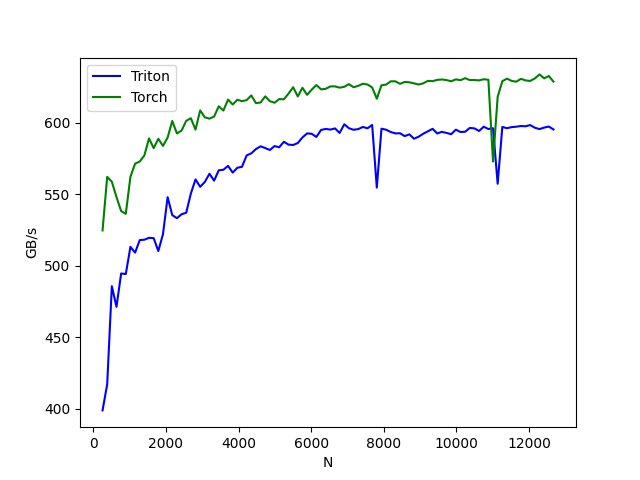
矩阵乘法的实现示例代码如下:
import torch
import triton
import triton.language as tl
import time

# Define matrix multiplication kernel using Triton
@triton.jit
def matmul_kernel(
    A, B, C, M, N, K, BLOCK_M: tl.constexpr, BLOCK_N: tl.constexpr, BLOCK_K: tl.constexpr,
):
    pid = tl.program_id(0)
    row = pid // (N // BLOCK_N)
    col = pid % (N // BLOCK_N)

    offs_m = row * BLOCK_M + tl.arange(0, BLOCK_M)
    offs_n = col * BLOCK_N + tl.arange(0, BLOCK_N)
    offs_k = tl.arange(0, BLOCK_K)

    a_ptrs = A + offs_m[:, None] * K + offs_k[None, :]
    b_ptrs = B + offs_k[:, None] * N + offs_n[None, :]

    accum = tl.zeros((BLOCK_M, BLOCK_N), dtype=tl.float32)

    for k in range(0, K, BLOCK_K):
        a = tl.load(a_ptrs)
        b = tl.load(b_ptrs)
        accum += tl.dot(a, b)
        a_ptrs += BLOCK_K
        b_ptrs += BLOCK_K * N

    c_ptrs = C + offs_m[:, None] * N + offs_n[None, :]
    tl.store(c_ptrs, accum)

def matmul(a, b):
    num_iters = 300
    M, K = a.shape
    N = b.shape[1]
    C = torch.zeros((M, N), dtype=torch.float32, device='cuda')

    # Compile and run Triton kernel
    grid = (M // 32, N // 32)

    start = time.time()
    print("[Matrix Multiply Using Triton] - Starting...")
    print(f"MatrixA({M},{K}), MatrixB({K},{N})")

    for _ in range(num_iters):
        matmul_kernel[grid](a, b, C, M, N, K, BLOCK_M=32, BLOCK_N=32, BLOCK_K=32)

    torch.cuda.synchronize()
    end = time.time()

    # Calculate performance metrics
    elapsed_time = end - start
    time_per_iteration = elapsed_time * 1000 / num_iters
    flops = 2.0 * M * N * K * num_iters
    gflops = (flops / elapsed_time) / 1e9

    # Output performance results
    print(f"Triton Performance= {gflops:.2f} GFlop/s, Time= {time_per_iteration:.3f} msec")
    return C

# Matrix sizes
M, N, K = 320, 320, 320

# Initialize matrices
A = torch.randn((M, K), dtype=torch.float16, device='cuda')
B = torch.randn((K, N), dtype=torch.float16, device='cuda')

# Call the matmul function
C = matmul(A, B)
print(f"Output matrix C: {C}")
结果:
[Matrix Multiply Using Triton] - Starting...
MatrixA(320,320), MatrixB(320,320)
Triton Performance= 79.84 GFlop/s, Time= 0.821 msec
Output matrix C: tensor([[  0.1220,  -4.0168, -11.4398,  ...,   1.5115,  -4.4500,  10.5483],
        [ 18.3915,  21.7275, -15.4414,  ...,  -8.9633,  32.6608,  27.5713],
        [-31.2961,   7.7287,   8.6794,  ...,  10.2873,  -3.2942,  26.0596],
        ...,
        [  0.0000,   0.0000,   0.0000,  ...,   0.0000,   0.0000,   0.0000],
        [  0.0000,   0.0000,   0.0000,  ...,   0.0000,   0.0000,   0.0000],
        [  0.0000,   0.0000,   0.0000,  ...,   0.0000,   0.0000,   0.0000]],
       device='cuda:0')
框架模型层
Triton 可以与 PyTorch 框架无缝集成,虽然 PyTorch 模型不会直接转换为 Triton,但可以利用 Triton 编写自定义的 CUDA 核心,从而优化特定的操作。这种方式让开发者可以在 PyTorch 中使用 Triton 优化的操作,提升性能。
例如,在 PyTorch 模型中包装 Triton 核心的代码:
class MyModel(torch.nn.Module):
    def forward(self, x, y):
        z = triton_add_wrapper(x, y)
        return z
Unsloth 是一个高效的库,使用 Triton 编写的算子,能够实现高性能的模型训练和推理,且没有准确性损失。下面是使用 Unsloth 的 FastLanguageModel 来加载一个预训练的 LLaMA 3 模型并进行推理的示例代码:
import time
import torch
from unsloth import FastLanguageModel

max_seq_length = 2048 # Choose any! We auto support RoPE Scaling internally!
dtype = None # None for auto detection. Float16 for Tesla T4, V100, Bfloat16 for Ampere+
load_in_4bit = True # Use 4bit quantization to reduce memory usage. Can be False.

model, tokenizer = FastLanguageModel.from_pretrained(
    model_name = "/home/aii-works/llama3/Meta-Llama-3-8B-Instruct",
    max_seq_length = max_seq_length,
    dtype = dtype,
    load_in_4bit = load_in_4bit
)

model = FastLanguageModel.get_peft_model(
    model,
    r = 16, # Choose any number > 0 ! Suggested 8, 16, 32, 64, 128
    target_modules = ["q_proj", "k_proj", "v_proj", "o_proj",
                      "gate_proj", "up_proj", "down_proj",],
    lora_alpha = 16,
    lora_dropout = 0, # Supports any, but = 0 is optimized
    bias = "none",    # Supports any, but = "none" is optimized
    # [NEW] "unsloth" uses 30% less VRAM, fits 2x larger batch sizes!
    use_gradient_checkpointing = "unsloth", # True or "unsloth" for very long context
    random_state = 3407,
    use_rslora = False,  # We support rank stabilized LoRA
    loftq_config = None, # And LoftQ
)

alpaca_prompt = """Below is an instruction that describes a task, paired with an input that provides further context. Write a response that appropriately completes the request.

### Instruction:
{}

### Input:
{}

### Response:
{}"""

FastLanguageModel.for_inference(model)

inputs = tokenizer(
[
    alpaca_prompt.format(
        # "Continue the fibonnaci sequence.", # instruction
        "Q:",
        "Name the planets in the solar system?",
        "", # output - leave this blank for generation!
    )
], return_tensors = "pt").to("cuda")

iterations = 10
with torch.no_grad():
    for _ in range(5):
        outputs = model.generate(**inputs, max_new_tokens = 64, use_cache = True)
t_start = time.time()
for _ in range(iterations):
    with torch.no_grad():
        outputs = model.generate(**inputs, max_new_tokens = 64, use_cache = True)
elapsed_time = time.time() - t_start
latency = elapsed_time / iterations * 1000
FPS = 1000 / latency

print(tokenizer.decode(outputs[0], skip_special_tokens=True))
print(f"FPS: {FPS:.2f}")
结果:
🦥 Unsloth: Will patch your computer to enable 2x faster free finetuning.
==((====))==  Unsloth 2024.8: Fast Llama patching. Transformers = 4.44.2.
   \\   /|    GPU: NVIDIA GeForce RTX 4080 SUPER. Max memory: 15.695 GB. Platform = Linux.
O^O/ \_/ \    Pytorch: 2.4.0. CUDA = 8.9. CUDA Toolkit = 12.1.
\        /    Bfloat16 = TRUE. FA [Xformers = 0.0.27.post2. FA2 = False]
 "-____-"     Free Apache license: http://github.com/unslothai/unsloth
Loading checkpoint shards: 100%|███████████████████████████████████████████████████████████████████████████████████████████████████████████████████████████████████████████████████████████████████████| 4/4 [00:02<00:00,  1.76it/s]
/home/aii-works/llama3/Meta-Llama-3-8B-Instruct does not have a padding token! Will use pad_token = <|reserved_special_token_250|>.
Unsloth 2024.8 patched 32 layers with 32 QKV layers, 32 O layers and 32 MLP layers.
huggingface/tokenizers: The current process just got forked, after parallelism has already been used. Disabling parallelism to avoid deadlocks...
To disable this warning, you can either:
        - Avoid using `tokenizers` before the fork if possible
        - Explicitly set the environment variable TOKENIZERS_PARALLELISM=(true | false)
Below is an instruction that describes a task, paired with an input that provides further context. Write a response that appropriately completes the request.

### Instruction:
Q:

### Input:
Name the planets in the solar system?

### Response:
The eight planets in our solar system, in order from the Sun, are:

1. Mercury
2. Venus
3. Earth
4. Mars
5. Jupiter
6. Saturn
7. Uranus
8. Neptune

Note: Pluto was previously considered a planet, but in 2006,
FPS: 0.89
Apache TVM (NVIDIA)
Apache TVM(Tensor Virtual Machine)是一个开源的深度学习编译器框架,旨在优化和部署机器学习模型到各种硬件平台,包括NVIDIA GPU。TVM在NVIDIA平台上的应用为开发者提供了强大的工具,以提高深度学习模型的性能和效率。
Apache TVM 概述
-
开源项目:TVM是Apache软件基金会的顶级项目。
-
端到端优化:从高级模型描述到低级硬件指令的全栈优化。
-
跨平台支持:支持多种硬件后端,包括CPU、GPU、FPGA等。
-
自动调优:使用机器学习技术自动优化张量运算。
TVM 在 NVIDIA 平台上的特点
-
CUDA 支持:TVM可以生成高效的CUDA代码,充分利用NVIDIA GPU的计算能力。
-
性能优化:通过自动调优和特定于NVIDIA架构的优化,提供卓越的性能。
-
灵活性:支持各种NVIDIA GPU架构,从消费级到数据中心级别的产品。
-
与NVIDIA生态系统集成:可以与NVIDIA的其他工具和库(如cuDNN)协同工作。
TVM 核心概念
-
计算图优化:优化深度学习模型的计算图结构。
-
调度原语:提供细粒度的控制来指定计算的执行方式。
-
自动调优:使用机器学习来搜索最佳的优化策略。
-
运行时:轻量级运行时支持模型的高效执行。
TVM 流程图
下图显示了 TVM 当前执行与优化过程:
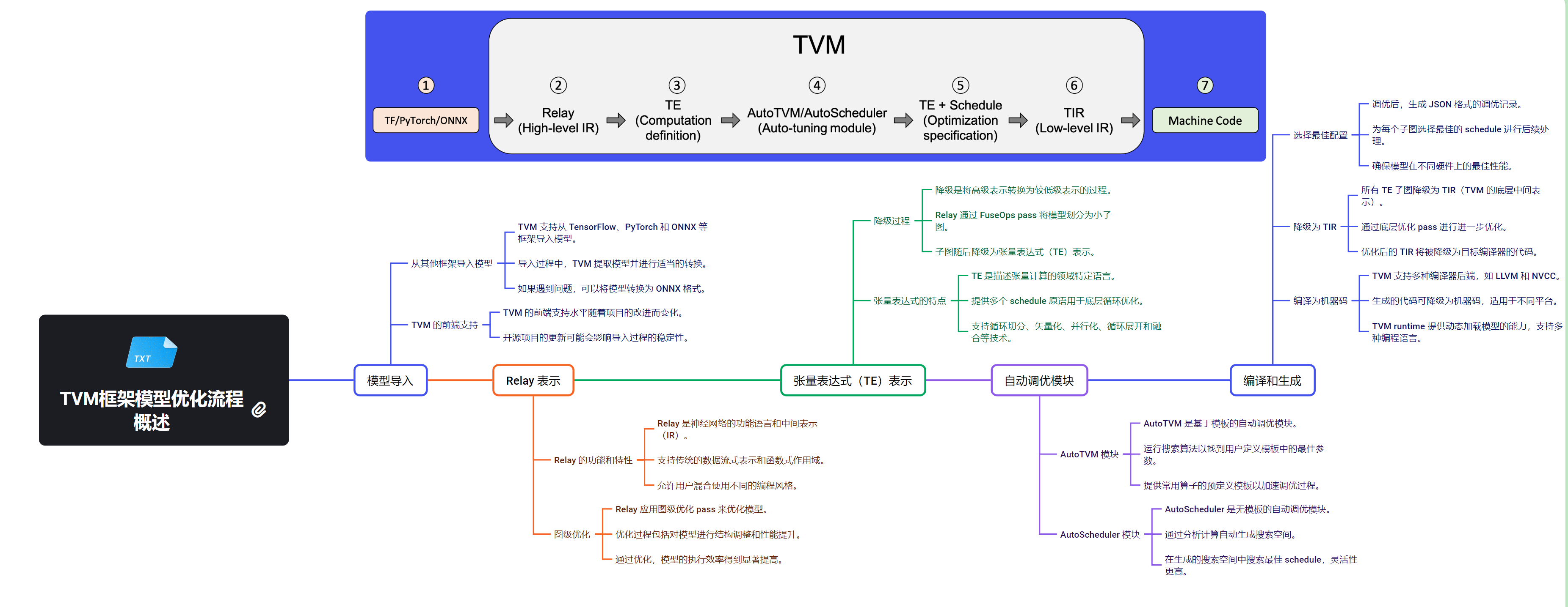
使用 TVM 的工作流程
- 导入预训练模型(如从PyTorch、TensorFlow等)
- 使用TVM编译和优化模型
- 在目标NVIDIA设备上进行自动调优
- 导出优化后的模型
- 在NVIDIA平台上部署和执行优化后的模型
TVM 支持的硬件概述
下图显示了 TVM 当前支持的硬件后端:

TVM vs 其他框架 on NVIDIA
-
vs CUDA:TVM生成CUDA代码,但提供了更高级的抽象和自动优化。
-
vs TensorRT:TVM提供更广泛的模型支持和更灵活的优化策略。
-
vs PyTorch/TensorFlow:TVM作为编译器,可以优化这些框架生成的模型。
TVM 在 NVIDIA 平台上的优势
-
性能提升:通过自动调优和特定于NVIDIA的优化,显著提高模型性能。
-
内存优化:更有效地利用GPU内存,支持更大的模型。
-
跨设备优化:同一模型可以针对不同的NVIDIA GPU架构进行优化。
-
自定义算子支持:轻松集成和优化自定义CUDA算子。
随着深度学习模型变得越来越复杂,TVM在NVIDIA平台上的重要性可能会进一步增加。它为开发者提供了一种强大的工具,以充分利用NVIDIA硬件的潜力,同时保持跨平台的灵活性。
Apache TVM为NVIDIA平台提供了一个强大的深度学习优化和部署解决方案。它结合了高性能、灵活性和易用性,使开发者能够充分发挥NVIDIA GPU的计算能力。随着AI和深度学习技术的不断发展,TVM有望在NVIDIA生态系统中扮演越来越重要的角色,推动更高效、更智能的计算解决方案的发展。
技术栈架构
1. 系统软件层
- CUDA Driver API:低级 API,提供对 NVIDIA GPU 的直接控制
- 允许直接管理设备、内存分配和程序执行
- 适用于需要细粒度控制的高级应用
- 为 TVM 提供与 NVIDIA GPU 硬件交互的底层接口
- TVM Compiler Infrastructure:TVM 的编译器基础设施
- 支持多种硬件后端,包括 CUDA 设备
- 提供了一个灵活的编译流程,可针对不同硬件进行优化
2. 运行时环境层
- CUDA Runtime API:高级 API,简化了 GPU 编程,自动管理许多底层细节
- 为 TVM 提供更高级的抽象,简化了 GPU 的使用
- 自动处理上下文管理和程序加载等任务
- TVM Runtime:TVM 框架的运行时环境
- 管理 TVM 编译的模型的执行
- 支持多种硬件后端,包括 CUDA 设备
- 与 CUDA Runtime API 集成,提供对 NVIDIA GPU 的支持
3. 编程模型和语言层
- CUDA C/C++:扩展了 C/C++ 语言,允许开发者编写在 GPU 上运行的并行程序
- 为 TVM 提供了一种与 NVIDIA GPU 交互的编程方式
- 可与 TVM DSL 结合使用,实现对 CUDA 设备的优化
- TVM DSL:TVM 提供的领域特定语言
- 用于描述和优化机器学习模型
- 提供了一种声明式的方式来表达计算
- 可以针对 CUDA 设备等不同硬件后端进行优化
4. 计算库层
- cuBLAS:用于线性代数计算的库
- 提供 GPU 加速的矩阵运算和 BLAS 功能
- 可与 TVM Relay 集成,实现对 CUDA 设备的优化
- NCCL:用于多 GPU 通信的库
- 支持多 GPU 之间的高效通信和数据交换
- 可与 TVM 结合使用,支持分布式深度学习训练
- TVM Relay:TVM 的高级编程接口
- 提供了一种声明式的方式来表达机器学习模型
- 支持针对 CUDA 设备等不同硬件的优化编译
5. 框架模型层
- PyTorch with TVM:利用 TVM 优化 PyTorch 模型在 CUDA 设备上的性能
- TensorFlow with TVM:利用 TVM 优化 TensorFlow 模型在 CUDA 设备上的性能
- 其他基于 TVM 的深度学习框架集成
- 通过 TVM 实现对 CUDA 设备的高性能优化
关系解析
TVM作为一个灵活的深度学习编译器框架,与PyTorch深度集成,通过自定义算子、JIT编译和GPU内核融合等技术,大幅提升了PyTorch模型在GPU上的执行效率。同时,TVM还利用CUDA Runtime API和CUDA Driver API,实现了对GPU硬件的精细控制和优化,包括内存管理、设备操作和内核启动等。这种多层次的架构设计使TVM能够充分发挥GPU的计算能力,同时为开发者提供了一个高度灵活和易用的工具。此外,TVM还提供了自己的运行时环境TVM Runtime,以及用于部署的TVM Relay和TVM DSL等组件,形成了一个完整的深度学习加速生态系统。通过整合这些技术,TVM为开发者带来了显著的性能提升,同时简化了高性能深度学习应用的开发过程。
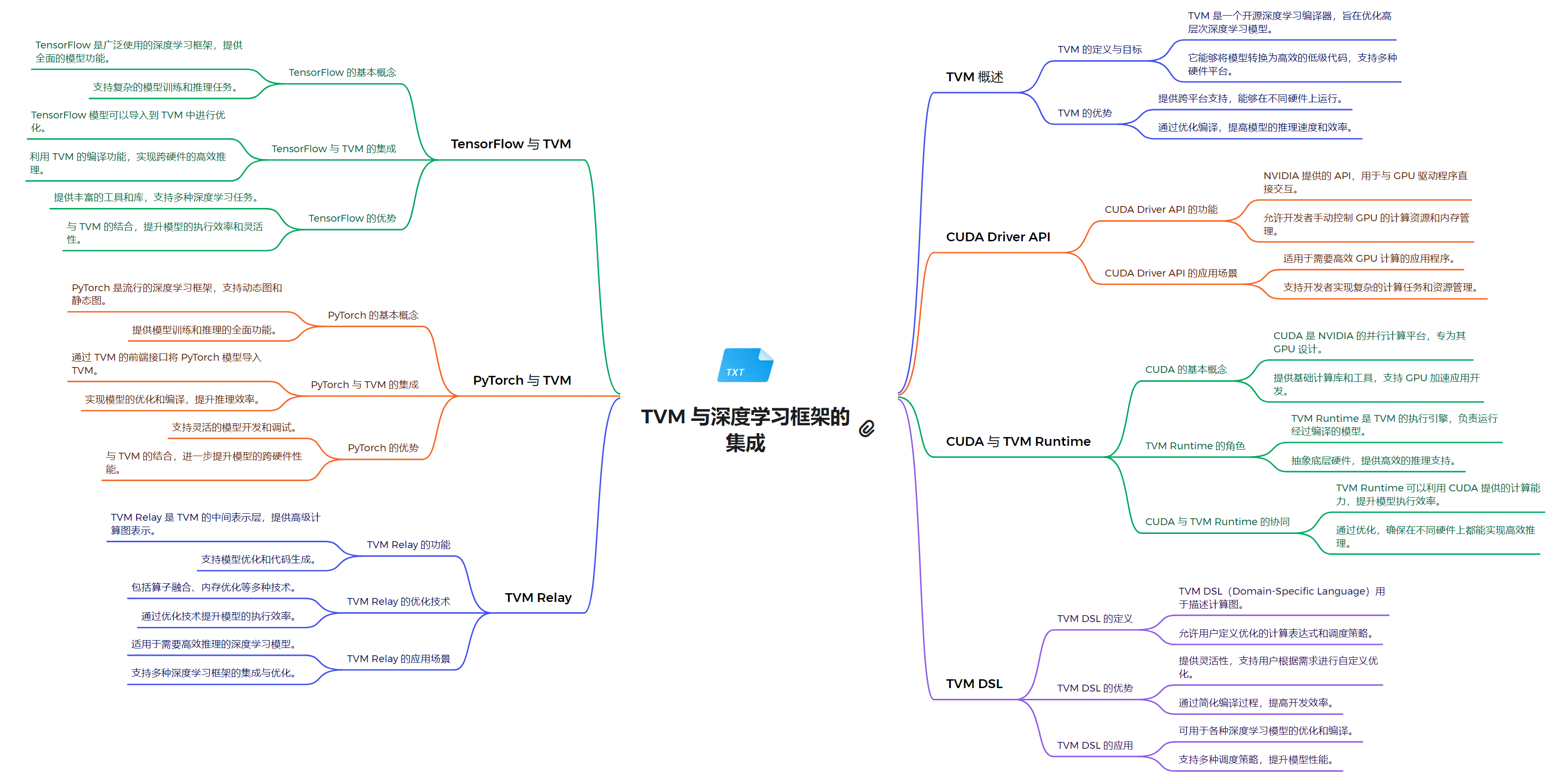
系统软件层
TVM 通过使用 CUDA Driver API 与底层 GPU 进行交互的具体流程可以总结为以下几个步骤:
-
在 TVM 中,首先通过 CUDA Driver API 初始化 GPU 上下文 (
cuCtxCreate或者cuCtxSetCurrent)。这个上下文用于管理与特定 GPU 设备的交互,并确保后续的 GPU 操作在这个上下文中执行。 -
在 GPU 上分配内存,TVM 通过调用
cuMemAlloc来请求 GPU 显存,以存储计算所需的输入、输出及中间结果数据。可以使用cuMemFree来释放不再使用的显存。 -
TVM 需要将数据从主机(CPU)传输到设备(GPU)。通过调用
cuMemcpyHtoD(从主机到设备)和cuMemcpyDtoH(从设备到主机)进行数据传输。 -
使用
cuModuleGetFunction获取 CUDA 函数句柄,通过cuLaunchKernel启动内核执行。启动时可以指定线程块和线程网格的配置,这样可以充分利用 GPU 的并行计算能力。 -
为了确保所有的 GPU 操作都完成,可以使用
cuCtxSynchronize,它会等待所有在当前上下文中发起的操作执行完毕。 -
当 GPU 计算任务完成之后,TVM 会通过调用相应的 CUDA Driver API 函数来释放内存和资源,包括
cuMemFree和cuModuleUnload,以避免内存泄漏。
运行时环境层
编写了一个程序,列出系统中可用的 CUDA 设备,获取设备的名称、计算能力和全局内存大小等信息。
- 检查 CUDA 设备: 定义
check_cuda函数以尝试获取第一个 CUDA 设备并收集其信息。 - 获取设备信息: 包括计算能力、最大线程数、共享内存等。
- 异常处理: 捕获并打印获取设备信息时的错误。
- 输出设备信息: 打印设备的详细信息和名称。
代码:
import tvm
from tvm.contrib import nvcc

# 检查 TVM 是否支持 CUDA 并返回设备详细信息
def check_cuda():
    try:
        # 尝试获取 CUDA 设备
        device = tvm.cuda(0)

        # 获取设备的详细信息
        device_info = {
            "compute_capability": device.compute_version,  # 计算能力
            "max_threads_per_block": device.max_threads_per_block,  # 每个块的最大线程数
            "max_shared_memory_per_block": device.max_shared_memory_per_block,  # 每个块的最大共享内存
            "multi_processor_count": device.multi_processor_count,  # 多处理器数量
            "warp_size": device.warp_size,  # warp 大小
            "total_global_memory": device.total_global_memory,  # 总全局内存
        }
        print("CUDA check success")
        print("Device Info:")
        for key, value in device_info.items():
            print(f"  {key}: {value}")
        return device_info
    except Exception as e:
        print(f"CUDA check failed: {e}")
        return None

check_cuda()

# 获取当前可用的设备
dev = tvm.cuda(0)  # 获取第一个 GPU 设备

# 输出设备名称
device_name = dev.device_name
print("Device Name:", device_name)

# 获取设备的详细信息
device_info = {
    "Device Type": dev.device_type,
    "Device ID": dev.device_id,  # 使用 device_id 替代 device_index
}
# 输出设备详细信息
for key, value in device_info.items():
    print(f"{key}: {value}")
结果:
CUDA check success
Device Info:
  compute_capability: 8.9
  max_threads_per_block: 1024
  max_shared_memory_per_block: 49152
  multi_processor_count: 80
  warp_size: 32
  total_global_memory: 16852844544
Device Name: NVIDIA GeForce RTX 4080 SUPER
Device Type: 2
Device ID: 0
编程模型和语言层
TVM 是一个专注于深度学习模型优化和编译的开源框架,它的编程模型基于 Tensor 表达、算子(Operator)定义 和 调度(Schedule),并且通过高效代码生成实现硬件上的高性能计算。TVM 编程模型的关键步骤包括:
- 定义计算:使用 TVM 的计算表达式定义要执行的计算任务。
- 调度(Scheduling):为计算任务安排执行顺序和资源分配,指定如何并行化、向量化等。
- 编译:将计算和调度方案编译为可在目标硬件上运行的代码。
- 执行:在目标设备上运行编译后的代码。
下面是一个简单的示例,它展示了TVM的基本编程流程,包括定义矩阵加法运算并在CPU或者GPU上执行。
TVM 的编程模型示例
import tvm
from tvm import te
import numpy as np

# 1. 定义计算:A 和 B 矩阵相加,生成 C
n = te.var("n")
A = te.placeholder((n,), name="A")
B = te.placeholder((n,), name="B")
C = te.compute(A.shape, lambda i: A[i] + B[i], name="C")

# 2. 创建调度:默认调度会按顺序执行计算
s = te.create_schedule(C.op)

# 3. 编译:为 GPU 生成低级代码
target = "llvm"  # CPU 目标 如果是hi是GPU上执行则改为“cuda”
fadd = tvm.build(s, [A, B, C], target, name="matrix_add")

# 4. 在 TVM 运行时中执行
ctx = tvm.cpu(0)
n_value = 1024
a = tvm.nd.array(np.random.uniform(size=n_value).astype(A.dtype), ctx)
b = tvm.nd.array(np.random.uniform(size=n_value).astype(B.dtype), ctx)
c = tvm.nd.array(np.zeros(n_value, dtype=C.dtype), ctx)

# 调用编译好的函数
fadd(a, b, c)

# 检查结果
np.testing.assert_allclose(c.asnumpy(), a.asnumpy() + b.asnumpy())
print("Result matches with NumPy calculation.")
代码解释
-
定义计算:
- 使用
te.placeholder创建两个占位符A和B,分别代表输入的矩阵。 - 使用
te.compute定义计算表达式,这里表示逐元素对A和B执行加法操作,结果存储在C中。
- 使用
-
调度计算:
- 使用
te.create_schedule(C.op)创建调度。这里使用的是默认的顺序执行调度,也可以通过优化调度提升性能。
- 使用
-
编译代码:
- 使用
tvm.build函数,将计算和调度编译成针对指定目标(如 CPU 或 GPU)的可执行代码。
- 使用
-
运行并验证结果:
- 创建 TVM 的
nd.array将 NumPy 数据传入 TVM 中运行。 - 使用编译好的函数
fadd进行计算,并验证结果是否与 NumPy 计算的结果一致。 结果
- 创建 TVM 的
Result matches with NumPy calculation.
这个简单的例子展示了 TVM 的核心编程流程。在实际的深度学习模型优化中,TVM 提供了更多高级特性,例如自动调度(AutoScheduler)、多目标硬件支持(CPU、GPU、TPU)等,可以极大提升模型在不同硬件平台上的运行效率。
下面再给一个 TVM 示例,这次展示如何使用 TVM 优化二维矩阵乘法(矩阵乘法是深度学习中常见的操作之一),并进行简单的调度优化。
TVM 矩阵乘法示例
import tvm
from tvm import te
import numpy as np

# 1. 定义矩阵乘法计算: C[i, j] = sum(A[i, k] * B[k, j] for k in range(K))
N = te.var("N")
M = te.var("M")
K = te.var("K")

# 定义矩阵 A, B
A = te.placeholder((N, K), name="A")
B = te.placeholder((K, M), name="B")

# 定义矩阵乘法的计算
C = te.compute((N, M), lambda i, j: te.sum(A[i, k] * B[k, j] for k in range(K)), name="C")

# 2. 创建调度
s = te.create_schedule(C.op)

# 简单调度优化:并行化行方向上的计算
# 这是 TVM 调度中常见的优化方式
s[C].parallel(C.op.axis[0])

# 3. 编译:为 CPU 生成代码
target = "llvm"  # CPU 目标
fmatmul = tvm.build(s, [A, B, C], target, name="matrix_multiply")

# 4. 在 TVM 运行时中执行
ctx = tvm.cpu(0)

# 定义矩阵的大小
N_value = 1024
M_value = 1024
K_value = 1024

# 创建随机的输入矩阵 A 和 B
a = tvm.nd.array(np.random.uniform(size=(N_value, K_value)).astype(A.dtype), ctx)
b = tvm.nd.array(np.random.uniform(size=(K_value, M_value)).astype(B.dtype), ctx)
c = tvm.nd.array(np.zeros((N_value, M_value), dtype=C.dtype), ctx)

# 调用编译好的矩阵乘法函数
fmatmul(a, b, c)

# 使用 NumPy 计算参考结果
np_c = np.dot(a.asnumpy(), b.asnumpy())

# 验证 TVM 计算的结果是否与 NumPy 的结果一致
np.testing.assert_allclose(c.asnumpy(), np_c, rtol=1e-5)
print("Matrix multiplication result matches with NumPy.")
代码解释
-
定义矩阵乘法:
- 使用
te.placeholder创建两个占位符A和B,分别代表输入的二维矩阵。 - 使用
te.compute定义矩阵乘法,te.sum用于对中间维度K进行求和,从而实现矩阵乘法的核心计算。
- 使用
-
调度优化:
- 使用
te.create_schedule(C.op)创建调度方案。 - 通过
s[C].parallel(C.op.axis[0])让 TVM 并行化行方向上的计算,这是一个简单的优化方法,用于利用多核 CPU 提升矩阵乘法的性能。
- 使用
-
编译代码:
- 使用
tvm.build将计算和调度方案编译成可执行的 CPU 代码。
- 使用
-
运行并验证结果:
- 创建随机的矩阵
A和B,在 TVM 的运行时环境中执行编译好的矩阵乘法函数。 - 使用 NumPy 的
dot函数计算参考矩阵乘法的结果,并与 TVM 的结果进行比较,确保其一致性。
- 创建随机的矩阵
结果
Matrix multiplication result matches with NumPy.
这表明 TVM 编译后的矩阵乘法操作正确地执行,并且与 NumPy 的计算结果一致。
计算库层
TVM 仓库的根目录包含以下几个子目录:
- src:存放用于算子编译和部署运行时的 C++ 代码。
- src/relay:实现了 Relay,这是一个为深度学习框架提供的新功能 IR。
- python:提供 Python 前端,用于封装 src 中实现的 C++ 函数和对象。
- src/topi:定义标准神经网络算子的计算和后端调度。
src/relay 是负责管理计算图的组件,其中图结构中的节点通过 src 其余部分提供的基础设施进行编译和执行。python 为 C++ API 和执行编译的驱动代码提供了 Python 绑定。与节点对应的算子在 src/relay/op 中注册,而算子的实现则在 topi 中,使用的编程语言包括 C++ 和 Python。
其中:
- IR(Intermediate Representation):一种中间表示形式,用于编译过程中的高级代码表示。
- 算子(Operator):在深度学习中,算子通常指代执行特定计算的函数,比如卷积、矩阵乘等。
- 调度(Schedule):定义了算子如何在硬件上执行的策略,包括循环的嵌套结构、并行化、向量化等。
向量加法示例:
n = 1024
A = tvm.te.placeholder((n,), name='A')
B = tvm.te.placeholder((n,), name='B')
C = tvm.te.compute(A.shape, lambda i: A[i] + B[i], name="C")
在 python/tvm/te/tensor.py 中定义的 A、B 和 C 的类型都是 tvm.tensor.Tensor。这些 Python Tensor 是由 C++ Tensor 支持的,其实现位于 include/tvm/te/tensor.h 和 src/te/tensor.cc 文件中。在 TVM 中,所有的 Python 类型都可以视为与其底层 C++ 类型具有相同名称的句柄。
从以下 Python Tensor 类型的定义中可以看出,tvm.tensor.Tensor 是 Object 的一个子类。
@register_object
class Tensor(Object, _expr.ExprOp):
    """Tensor object, to construct, see function.Tensor"""

    def __call__(self, *indices):
       ...
-
在 TVM 中,每个
Tensor对象都有一个与之关联的Operation对象。Tensor是在计算过程中存储数据的多维数组,而Operation表示对一个或多个Tensor进行操作的计算。这两个概念在代码中有明确的实现,相关定义分别在python/tvm/te/tensor.py、include/tvm/te/operation.h和src/tvm/te/operation目录下。 -
每个
Tensor对象都可以看作是其相应的Operation的输出,这意味着通过执行某个Operation可以生成一个Tensor。 -
Operation对象提供了一个input_tensors()方法,这个方法返回一个输入Tensor的列表。这使得开发者能够跟踪不同Operation之间的依赖关系,了解一个Operation需要哪些输入Tensor,以及这些输入Tensor是由哪些其他Operation产生的。 -
在计算图中,当我们想要调度某个计算时,需要将输出张量(例如上面提到的
C张量)对应的Operation对象传递给python/tvm/te/schedule.py中的tvm.te.create_schedule()函数create_schedule()函数负责生成计算的调度策略,以优化计算的执行。这是构建高效计算图的重要步骤,因为它允许对计算的执行顺序和方式进行控制,从而提高性能。
S = tvm.te.create_schedule(C.op)
函数被映射到 include/tvm/schedule.h 中的 C++ 函数。
inline Schedule create_schedule(Array<Operation> ops) {
    return Schedule(ops);
}
-
在 TVM 中,调度由多个
Stage和输出的Operation组成。每个Stage代表一个Operation的计算过程。 -
以“向量加法”(Vector Add)为例,假设有两个占位符
Operation和一个计算Operation,那么这个调度(s)将包含三个阶段(Stage)。 -
每个
Stage存储有关循环嵌套的信息,包括:循环嵌套结构:描述了如何将计算划分为多个循环的结构。循环类型:标识每个循环的执行方式,比如:Parallel(并行):表示该循环可以在多个线程中并行执行。Vectorized(向量化):表示该循环将数据分块处理,以提高效率。Unrolled(展开):表示将循环展开为多个相同的操作,以减少循环开销。位置:指明在下一个Stage的循环嵌套中执行该计算的位置(如果有嵌套的话)。create_schedule() 函数的作用:create_schedule()函数用于创建默认的调度。这个调度提供了基础的计算顺序和结构。默认的调度通常会调用tvm.build(...)函数来生成可执行的代码。 -
为了使调度可以在 GPU 上运行,需要为调度中的
Stage绑定必要的线程。这一步骤是非常重要的,因为 GPU 的并行计算能力依赖于对线程的有效管理和分配。 -
通过线程绑定,开发者可以控制计算的并行性,从而充分利用 GPU 的硬件资源,以实现更高的性能。
target = "cuda"
bx, tx = s[C].split(C.op.axis[0], factor=64)
s[C].bind(bx, tvm.te.thread_axis("blockIdx.x"))
s[C].bind(tx, tvm.te.thread_axis("threadIdx.x"))
fadd = tvm.build(s, [A, B, C], target)
target = "cuda"指定了目标平台是CUDA,意味着生成的代码将在GPU上运行。split和bind是调度操作,用于优化并行执行。split将计算操作的循环分割成更小的部分,bind将这些分割的部分绑定到GPU的线程和块上。tvm.build函数接受调度、输入和输出Tensor以及目标平台,然后返回一个可以在该平台上运行的模块。
tvm.build() 函数:
-
tvm.build()函数定义在python/tvm/driver/build_module.py中。它的主要作用是接收一个调度(schedule)、输入和输出的Tensor,以及一个目标设备(target),然后返回一个tvm.runtime.Module对象。返回的tvm.runtime.Module对象包含一个可以通过函数调用的已编译函数,这意味着用户可以直接调用这个编译后的函数进行计算,而无需关心底层实现细节。 -
tvm.build()的过程可以分为两个主要步骤:降级:降级过程将高级、初始的循环嵌套结构转化为最终的底层中间表示(IR)。这一过程是由tvm.lower()函数完成的,tvm.lower()也定义在python/tvm/build_module.py中。降级的第一步是进行边界推断,确定每个循环的迭代范围,以便在生成 IR 时确保计算的正确性。随后,tvm.lower()会创建一个初始的循环嵌套结构,以便更好地表达计算的逻辑和顺序。代码生成:在降级完成后,接下来的步骤是根据底层的 IR 生成目标机器代码。这一过程涉及将 IR 转换为特定硬件可以理解和执行的机器代码。 -
降级的过程有助于将更高级的计算抽象(例如高层的循环结构和调度策略)转化为更为底层的表示,使得后续的代码生成过程能够更加有效地针对特定硬件进行优化。通过将计算表示降级到 IR,TVM 能够更灵活地进行优化并适配多种硬件目标
def lower(sch,
          args,
          name="default_function",
          binds=None,
          simple_mode=False):
   ...
   bounds = schedule.InferBound(sch)
   stmt = schedule.ScheduleOps(sch, bounds)
   ...
边界推断(Bound Inference):
- 边界推断是一个关键的过程,它用于推断所有循环的边界和中间缓冲区的大小。这对于生成有效的代码和优化计算非常重要。
- 如果目标是 CUDA 后端,并且使用了共享内存,边界推断将自动确定所需的最小共享内存尺寸。这一过程确保了在运行时可以有效利用共享内存,从而提高计算性能。
边界推断的实现:边界推断的实现代码位于以下文件中:
-
src/te/schedule/bound.cc -
src/te/schedule/graph.cc -
src/te/schedule/message_passing.cc -
这些实现文件负责具体的边界推断算法和逻辑,包括如何根据调度信息推断出循环的边界和缓冲区的大小。
ScheduleOps() 的作用:
stmt是ScheduleOps()函数的输出,表示一个初始的循环嵌套结构。这个结构是调度的基础,反映了计算中循环的组织方式。- 如果调度过程中已经应用了
reorder或split等原语,则stmt将反映这些变化,确保生成的初始循环结构与应用的调度操作一致。 ScheduleOps()函数的定义位于src/te/schedule/schedule_ops.cc中。
接下来,对 stmt 在 src/tir/pass 子目录下进行降级处理。
...
stmt = ir_pass.VectorizeLoop(stmt)
...
stmt = ir_pass.UnrollLoop(
    stmt,
    cfg.auto_unroll_max_step,
    cfg.auto_unroll_max_depth,
    cfg.auto_unroll_max_extent,
    cfg.unroll_explicit)
...
-
在降级完成后,
build()函数负责从降级后的函数生成特定目标的机器代码。这一步是将中间表示(IR)转化为实际可执行的代码。 -
如果目标是 x86 架构,生成的代码将包含 SSE(Streaming SIMD Extensions)或 AVX(Advanced Vector Extensions)指令,以优化计算性能。
-
如果目标是 CUDA,生成的代码将包含 PTX(Parallel Thread Execution)指令,这是 NVIDIA 的一种中间表示,用于描述并行计算的指令。
-
除了生成目标专用的机器代码,TVM 还会生成一段宿主机代码。这部分代码负责执行一些重要的任务,如内存管理和内核启动等。宿主机代码确保了生成的内核能够在目标设备上正确运行并管理资源。
-
代码生成的具体实现是在
build_module()函数中完成的,该函数定义在python/tvm/target/codegen.py中。这个 Python 函数负责协调代码生成的各个环节。 -
在 C++ 端,代码生成的实现细节位于
src/target/codegen子目录中。这里包含了许多与代码生成相关的实现和优化。 -
build_module()函数最终会调用 C++ 端的Build()函数,后者位于src/target/codegen/codegen.cc中。Build()函数负责将具体的代码生成逻辑实现,完成从中间表示到目标机器代码的转换。
TVM_REGISTER_GLOBAL("codegen.build_cuda")
.set_body([](TVMArgs args, TVMRetValue* rv) {
    *rv = BuildCUDA(args[0]);
});
-
BuildCUDA()函数使用定义在src/codegen/codegen_cuda.cc中的CodeGenCUDA类,从降级的 IR(中间表示)中生成 CUDA 内核源代码。这意味着它将高层的计算表示转化为适合在 NVIDIA GPU 上执行的 CUDA 代码。 -
生成的 CUDA 内核源代码随后通过 NVRTC(NVIDIA Runtime Compilation)进行编译。NVRTC 是 NVIDIA 提供的一个库,允许在运行时编译 CUDA 程序,方便动态加载和执行。
-
如果目标是使用 LLVM 后端(如 x86、ARM、NVPTX 和 AMDGPU),代码生成主要由定义在
src/codegen/llvm/codegen_llvm.cc中的CodeGenLLVM类完成。 -
CodeGenLLVM的作用是将 TVM 的 IR 转换为 LLVM 的 IR。这一步是重要的,因为 LLVM 提供了强大的优化和代码生成能力。 -
在生成 LLVM IR 后,
CodeGenLLVM会执行一些 LLVM 优化。这些优化可以提高生成代码的性能,利用 LLVM 的优化工具链来提升最终机器代码的执行效率。 -
最后,
CodeGenLLVM会生成适用于特定目标架构的机器代码,使得该代码可以在不同的硬件上高效运行。
框架模型层
实现了一个使用tvm库进行矩阵乘法的 CUDA 程序。该程序在设备上执行矩阵乘法运算,并测量其性能。
- 包含必要的库和头文件,包括 CUDA 运行时库和辅助函数
- 定义矩阵乘法的维度: 设置矩阵 (A) 的大小为 (320* 640),矩阵 (B) 的大小为 (640* 320)。
- 构建计算图:使用
te.placeholder定义输入矩阵 (A) 和 (B)。使用te.compute定义输出矩阵 (C) 的计算逻辑,利用te.sum进行矩阵乘法。 - 创建调度:使用
te.create_schedule创建调度,并为 GPU 设置线程和块的调度。使用s[C].split和s[C].bind将计算任务分配到不同的 GPU 线程和块。 - 构建和运行函数
build_and_run:编译计算图为可执行的函数,并为输入矩阵分配随机数据。在设备上分配内存,创建 TVM 数组。计算 FLOPs,并在循环中执行矩阵乘法多次以计时。 - 计算性能指标:计算总运行时间和每秒浮点运算次数 (GFLOPS),并输出结果。
- 执行代码: 调用
build_and_run函数在 GPU 上执行矩阵乘法,并打印计算图的简化模式。
代码:
import tvm
from tvm import te
import numpy as np
import time

# 定义矩阵乘法的大小
M = 320
N = 640
K = 320

# 定义矩阵乘法
A = te.placeholder((M, N), name='A')
B = te.placeholder((N, K), name='B')
k = te.reduce_axis((0, N), name='k')
C = te.compute((M, K), lambda i, j: te.sum(A[i, k] * B[k, j], axis=k), name='C')

# 创建调度
s = te.create_schedule(C.op)

# GPU 线程调度
block_x = te.thread_axis("blockIdx.x")
block_y = te.thread_axis("blockIdx.y")
thread_x = te.thread_axis("threadIdx.x")
thread_y = te.thread_axis("threadIdx.y")

# 为 GPU 添加块和线程的调度
bx, tx = s[C].split(C.op.axis[0], factor=32)
by, ty = s[C].split(C.op.axis[1], factor=32)
s[C].bind(bx, block_x)
s[C].bind(by, block_y)
s[C].bind(tx, thread_x)
s[C].bind(ty, thread_y)

# 定义函数
def build_and_run(target_device="cuda", num_repeats=300):
    # 编译
    target = tvm.target.Target(target_device)
    f = tvm.build(s, [A, B, C], target=target, name='matmul')

    # 创建输入数据
    a_np = np.random.uniform(-1, 1, size=(M, N)).astype(np.float32)
    b_np = np.random.uniform(-1, 1, size=(N, K)).astype(np.float32)
    c_np = np.zeros((M, K), dtype=np.float32)

    # 在设备上分配内存
    dev = tvm.device(target_device, 0)
    a_tvm = tvm.nd.array(a_np, dev)
    b_tvm = tvm.nd.array(b_np, dev)
    c_tvm = tvm.nd.array(c_np, dev)

    # 计算 FLOPs(2 * M * N * K)
    flops = 2 * M * N * K

    # 运行并计时
    start_time = time.time()
    for i in range(num_repeats):
        f(a_tvm, b_tvm, c_tvm)
    dev.sync()  # 保证所有计算都已完成
    end_time = time.time()

    # 计算总时间和 GFLOPS
    total_time = end_time - start_time
    gflops = (flops * num_repeats) / (total_time * 1e9)

    # 输出结果
    print(f"Execution on {target_device} completed in {total_time:.4f} seconds for {num_repeats} iterations.")
    print(f"FLOPs: {flops} per matrix multiplication")
    print(f"GFLOPS: {gflops:.2f} GFLOPS")

# 在 GPU 上执行
build_and_run(target_device="cuda")
结果:
Execution on cuda completed in 0.1786 seconds for 300 iterations.
FLOPs: 131072000 per matrix multiplication
GFLOPS: 220.18 GFLOPS
实现了一个使用 TVM 的Auto-scheduling 进行算子优化。
- 定义一个带有偏置加法的矩阵乘法。这里使用了 TVM 张量表达式语言中的标准操作。区别在于函数定义上方使用了
register_workload装饰器。该函数应返回输入/输出张量列表。通过这些张量,auto-scheduler 可以得到整个计算图。 - 定义函数后,可以为 auto_scheduler 创建要搜索的任务。为这个矩阵乘法指定了特定的参数,如这里是两个大小为 1024x1024 的矩阵乘法。然后创建一个 N=L=M=1024 和 dtype="float32" 的搜索任务
num_measure_trials表示搜索过程中可用的测试试验次数。用RecordToFile将测试记录记录到文件matmul.json中。测试记录可用于查询历史最佳、恢复搜索以及以后进行更多分析。- auto-scheduling 完成后,可将 schedule 降级来查看 IR。auto-scheduler 执行合适的优化,包括多级循环切分、布局转换、并行化、向量化、循环展开和算子融合。
代码:
import logging
import sys
import numpy as np
import tvm
from tvm import te
import tvm.testing

from tvm import autotvm
@auto_scheduler.register_workload  # Note the auto_scheduler decorator
def matmul_add(N, L, M, dtype):
    A = te.placeholder((N, L), name="A", dtype=dtype)
    B = te.placeholder((L, M), name="B", dtype=dtype)
    C = te.placeholder((N, M), name="C", dtype=dtype)

    k = te.reduce_axis((0, L), name="k")
    matmul = te.compute(
        (N, M),
        lambda i, j: te.sum(A[i, k] * B[k, j], axis=k),
        name="matmul",
        attrs={"layout_free_placeholders": [B]},  # enable automatic layout transform for tensor B
    )
    out = te.compute((N, M), lambda i, j: matmul[i, j] + C[i, j], name="out")

    return [A, B, C, out]
target = tvm.target.Target("llvm")
N = L = M = 1024
task = tvm.auto_scheduler.SearchTask(func=matmul_add, args=(N, L, M, "float32"), target=target)

# 检查计算图
print("Computational DAG:")
print(task.compute_dag)
log_file = "matmul.json"
tune_option = auto_scheduler.TuningOptions(
    num_measure_trials=10,
    measure_callbacks=[auto_scheduler.RecordToFile(log_file)],
    verbose=2,
)
# 运行 auto-tuning(搜索)
task.tune(tune_option)
# 应用最佳 schedule
sch, args = task.apply_best(log_file)
print("Lowered TIR:")
print(tvm.lower(sch, args, simple_mode=True))
结果:
Computational DAG:
A = PLACEHOLDER [1024, 1024]
B = PLACEHOLDER [1024, 1024]
matmul(i, j) += (A[i, k]*B[k, j])
C = PLACEHOLDER [1024, 1024]
out(i, j) = (matmul[i, j] + C[i, j])
Lowered TIR:
@main = primfn(A_1: handle, B_1: handle, C_1: handle, out_1: handle) -> ()
  attr = {"from_legacy_te_schedule": True, "global_symbol": "main", "tir.noalias": True}
  buffers = {A: Buffer(A_2: Pointer(float32), float32, [1048576], []),
             B: Buffer(B_2: Pointer(float32), float32, [1048576], []),
             C: Buffer(C_2: Pointer(float32), float32, [1048576], []),
             out: Buffer(out_2: Pointer(float32), float32, [1048576], [])}
  buffer_map = {A_1: A, B_1: B, C_1: C, out_1: out}
  preflattened_buffer_map = {A_1: A_3: Buffer(A_2, float32, [1024, 1024], []), B_1: B_3: Buffer(B_2, float32, [1024, 1024], []), C_1: C_3: Buffer(C_2, float32, [1024, 1024], []), out_1: out_3: Buffer(out_2, float32, [1024, 1024], [])} {
  allocate(auto_scheduler_layout_transform: Pointer(global float32), float32, [1048576]), storage_scope = global {
    for (ax0.ax1.fused.ax2.fused: int32, 0, 128) "parallel" {
      for (ax4: int32, 0, 256) {
        for (ax6: int32, 0, 4) {
          for (ax7: int32, 0, 8) {
            auto_scheduler_layout_transform_1: Buffer(auto_scheduler_layout_transform, float32, [1048576], [])[((((ax0.ax1.fused.ax2.fused*8192) + (ax4*32)) + (ax6*8)) + ax7)] = B[((((ax4*4096) + (ax6*1024)) + (ax0.ax1.fused.ax2.fused*8)) + ax7)]
          }
        }
      }
    }
    for (i.outer.outer.j.outer.outer.fused: int32, 0, 16384) "parallel" {
      allocate(matmul: Pointer(global float32x8), float32x8, [4]), storage_scope = global;
      for (i.outer.inner: int32, 0, 2) {
        matmul_1: Buffer(matmul, float32x8, [4], [])[0] = broadcast(0f32, 8)
        matmul_1[1] = broadcast(0f32, 8)
        matmul_1[2] = broadcast(0f32, 8)
        matmul_1[3] = broadcast(0f32, 8)
        for (k.outer: int32, 0, 256) {
          for (k.inner: int32, 0, 4) {
            let cse_var_2: int32 = (((floormod(i.outer.outer.j.outer.outer.fused, 128)*8192) + (k.outer*32)) + (k.inner*8))
            let cse_var_1: int32 = ((((floordiv(i.outer.outer.j.outer.outer.fused, 128)*8192) + (i.outer.inner*4096)) + (k.outer*4)) + k.inner)
             {
              matmul_1[0] = (matmul_1[0] + (broadcast(A[cse_var_1], 8)*auto_scheduler_layout_transform_1[ramp(cse_var_2, 1, 8)]))
              matmul_1[1] = (matmul_1[1] + (broadcast(A[(cse_var_1 + 1024)], 8)*auto_scheduler_layout_transform_1[ramp(cse_var_2, 1, 8)]))
              matmul_1[2] = (matmul_1[2] + (broadcast(A[(cse_var_1 + 2048)], 8)*auto_scheduler_layout_transform_1[ramp(cse_var_2, 1, 8)]))
              matmul_1[3] = (matmul_1[3] + (broadcast(A[(cse_var_1 + 3072)], 8)*auto_scheduler_layout_transform_1[ramp(cse_var_2, 1, 8)]))
            }
          }
        }
        for (i.inner: int32, 0, 4) {
          let cse_var_3: int32 = ((((floordiv(i.outer.outer.j.outer.outer.fused, 128)*8192) + (i.outer.inner*4096)) + (i.inner*1024)) + (floormod(i.outer.outer.j.outer.outer.fused, 128)*8))
          out[ramp(cse_var_3, 1, 8)] = (matmul_1[i.inner] + C[ramp(cse_var_3, 1, 8)])
        }
      }
    }
  }
}
实现了在 Relay 中定义神经网络,并为装有 TVM 的 NVIDIA GPU 生成 runtime 库。
- 使用 Relay 框架定义了 ResNet18 神经网络模型,设定批量大小为 1,图像形状为 (3, 224, 224),输出类别数为 1000。
- 输出 ResNet18 模型的计算图结构,
show_meta_data=False表示不显示元数据。 - 设置优化级别为 3(包括算子融合、预计算、布局变换等优化),并指定 CUDA 作为目标设备,编译生成可在 GPU 上执行的库。
- 随机生成形状为
(1, 3, 224, 224)的输入数据。创建一个执行模块,并将输入数据设置到模型中,然后运行模型并获取输出结果。输出结果中的前 10 个元素。 - 使用 TVM 的
utils.tempdir创建临时目录,并将编译后的计算图、库和参数保存为文件,以便于后续部署时使用。 - 从保存的文件中加载编译模块,并使用相同的输入数据进行推理,获取输出结果。再次输出推理结果的前 10 个元素。
- 使用
tvm.testing.assert_allclose检查重新加载的模块输出与最初输出是否一致,容差设置为 1e-5。
import numpy as np
from tvm import relay
from tvm.relay import testing
import tvm
from tvm import te
from tvm.contrib import graph_executor
import tvm.testing
batch_size = 1
num_class = 1000
image_shape = (3, 224, 224)
data_shape = (batch_size,) + image_shape
out_shape = (batch_size, num_class)

mod, params = relay.testing.resnet.get_workload(
    num_layers=18, batch_size=batch_size, image_shape=image_shape
)

# 想显示元数据则设置 show_meta_data=True
#print(mod.astext(show_meta_data=False))
# 为 NVIDIA GPU 编译
opt_level = 3
target = tvm.target.cuda()
with tvm.transform.PassContext(opt_level=opt_level):
    lib = relay.build(mod, target, params=params)

#创建图执行器,然后在 NVIDIA GPU 上运行该模块
# create random input
dev = tvm.cuda()
data = np.random.uniform(-1, 1, size=data_shape).astype("float32")
# create module
module = graph_executor.GraphModule(lib["default"](dev))
# set input and parameters
module.set_input("data", data)
# run
module.run()
# get output
out = module.get_output(0, tvm.nd.empty(out_shape)).numpy()

# Print first 10 elements of output
print(out.flatten()[0:10])
结果:
[0.00089283 0.00103331 0.0009094  0.00102275 0.00108751 0.00106737
 0.00106262 0.00095838 0.00110792 0.00113151]
# create random input 图执行器,然后在 NVIDIA GPU 上运行该模块

dev = tvm.cuda()
data = np.random.uniform(-1, 1, size=data_shape).astype("float32")

# create module
module = graph_executor.GraphModule(lib["default"](dev))

# set input and parameters
module.set_input("data", data)

# run
module.run()

# get output
out = module.get_output(0, tvm.nd.empty(out_shape)).numpy()

# Print first 10 elements of output
print(out.flatten()[0:10])
结果:
[0.00089283 0.00103331 0.0009094  0.00102275 0.00108751 0.00106737
 0.00106262 0.00095838 0.00110792 0.00113151]
# 保存和加载编译模块 分别将计算图、库和参数保存到不同文件

from tvm.contrib import utils

temp = utils.tempdir()
path_lib = temp.relpath("deploy_lib.tar")
lib.export_library(path_lib)
print(temp.listdir())

# 重新加载模块
loaded_lib = tvm.runtime.load_module(path_lib)
input_data = tvm.nd.array(data)
module = graph_executor.GraphModule(loaded_lib["default"](dev))
module.run(data=input_data)
out_deploy = module.get_output(0).numpy()

# 打印输出的前十个元素
print(out_deploy.flatten()[0:10])

# 检查来自部署模块的输出和原始输出是否一致
tvm.testing.assert_allclose(out_deploy, out, atol=1e-5)
结果:
['deploy_lib.tar']

[0.00089283 0.00103331 0.0009094  0.00102275 0.00108751 0.00106737
 0.00106262 0.00095838 0.00110792 0.00113151]
实现了将 ONNX 模型编译到 TVM Runtime并使用 TVMC 运行来自编译模块的模型
- 从指定的 URL 下载图像,并保存为
imagenet_cat.png。 - 使用 PIL 库将下载的图像大小调整为 224x224,以适应标准的图像输入要求(例如 ResNet)。
- 将图像数据从 HWC(Height-Width-Channel)格式转换为 NCHW(Channel-Height-Width)格式,这是 ONNX 模型的输入格式要求。
- 根据 ImageNet 的标准化方法,对图像进行归一化处理,减去均值
imagenet_mean并除以标准差imagenet_stddev。 - 将图像数据扩展一个维度,以符合神经网络模型所需的 batch 大小格式 (batch, channel, height, width)。
- 最终将预处理后的图像数据保存为
imagenet_cat.npz,用于后续推理。 - 从指定的 URL 下载 ImageNet 的类别标签列表,并保存为
synset.txt。 - 从保存的
predictions.npz文件中加载输出张量,该文件应是神经网络推理后的结果。 - 使用 softmax 函数将模型的输出转化为概率分布。根据概率分数对输出进行排序,选出排名前 5 的类别,并打印它们的标签及对应的概率。
from tvm.contrib.download import download_testdata
from PIL import Image
import numpy as np

img_url = "https://s3.amazonaws.com/model-server/inputs/kitten.jpg"
img_path = download_testdata(img_url, "imagenet_cat.png", module="data")

# 重设大小为 224x224
resized_image = Image.open(img_path).resize((224, 224))
img_data = np.asarray(resized_image).astype("float32")

# ONNX 需要 NCHW 输入, 因此对数组进行转换
img_data = np.transpose(img_data, (2, 0, 1))

# 根据 ImageNet 进行标准化
imagenet_mean = np.array([0.485, 0.456, 0.406])
imagenet_stddev = np.array([0.229, 0.224, 0.225])
norm_img_data = np.zeros(img_data.shape).astype("float32")
for i in range(img_data.shape[0]):
      norm_img_data[i, :, :] = (img_data[i, :, :] / 255 - imagenet_mean[i]) / imagenet_stddev[i]

# 添加 batch 维度
img_data = np.expand_dims(norm_img_data, axis=0)

# 保存为 .npz(输出 imagenet_cat.npz)
np.savez("imagenet_cat", data=img_data)

import os.path
import numpy as np

from scipy.special import softmax

from tvm.contrib.download import download_testdata

# 下载标签列表
labels_url = "https://s3.amazonaws.com/onnx-model-zoo/synset.txt"
labels_path = download_testdata(labels_url, "synset.txt", module="data")

with open(labels_path, "r") as f:
    labels = [l.rstrip() for l in f]

output_file = "predictions.npz"

# 打开并读入输出张量
if os.path.exists(output_file):
    with np.load(output_file) as data:
        scores = softmax(data["output_0"])
        scores = np.squeeze(scores)
        ranks = np.argsort(scores)[::-1]

        for rank in ranks[0:5]:
            print("class='%s' with probability=%f" % (labels[rank], scores[rank]))
结果:
class='n02123045 tabby, tabby cat' with probability=0.621104
class='n02123159 tiger cat' with probability=0.356378
class='n02124075 Egyptian cat' with probability=0.019712
class='n02129604 tiger, Panthera tigris' with probability=0.001215
class='n04040759 radiator' with probability=0.000262
实现了使用 AutoTVM 在 TVM 中编译和优化 ONNX 模型。
-
使用
onnx.load()加载 ONNX 模型。 -
下载一张图像并将其调整为 224x224 像素,这是 ResNet 等模型的标准输入大小。根据 ImageNet 的标准对图像进行归一化,并调整为 NCHW 格式。
-
使用 Relay 前端编译模型,并指定目标架构(CUDA 用于 GPU)。
-
构建模型并将其转换为图模块以便执行。
-
使用 TVM 的运行时运行模型以获取预测结果,并使用 softmax 处理结果以获得每个类别的概率。
-
使用
timeit测量推理运行时间,并保存优化和未优化模型的结果。 -
使用 TVM 的 AutoTVM 中的
XGBTuner启动调优过程。 -
设置调优选项并在从模型中提取的任务上运行调优。
-
在调优后,使用在调优过程中找到的最佳配置重新构建模型,并验证优化模型的预测结果。
-
打印优化模型和未优化模型的性能指标以进行比较。
import onnx
from tvm.contrib.download import download_testdata
from PIL import Image
import numpy as np
import tvm.relay as relay
import tvm
from tvm.contrib import graph_executor

model_url = (
    "https://github.com/onnx/models/raw/main/"
    "vision/classification/resnet/model/"
    "resnet50-v2-7.onnx"
)

model_path = download_testdata(model_url, "resnet50-v2-7.onnx", module="onnx")
onnx_model = onnx.load(model_path)

img_url = "https://s3.amazonaws.com/model-server/inputs/kitten.jpg"
img_path = download_testdata(img_url, "imagenet_cat.png", module="data")

# 重设大小为 224x224

resized_image = Image.open(img_path).resize((224, 224))
img_data = np.asarray(resized_image).astype("float32")

# 输入图像是 HWC 布局,而 ONNX 需要 CHW 输入,所以转换数组

img_data = np.transpose(img_data, (2, 0, 1))

# 根据 ImageNet 输入规范进行归一化

imagenet_mean = np.array([0.485, 0.456, 0.406]).reshape((3, 1, 1))
imagenet_stddev = np.array([0.229, 0.224, 0.225]).reshape((3, 1, 1))
norm_img_data = (img_data / 255 - imagenet_mean) / imagenet_stddev

# 添加 batch 维度,期望 4 维输入:NCHW。

img_data = np.expand_dims(norm_img_data, axis=0)

# 为 numpy 的 RNG 设置 seed,得到一致的结果

np.random.seed(0)

target = "cuda"
# 可用 Netron 工具检查输入名称
input_name = "data"
shape_dict = {input_name: img_data.shape}

mod, params = relay.frontend.from_onnx(onnx_model, shape_dict)

with tvm.transform.PassContext(opt_level=3):
    lib = relay.build(mod, target=target, params=params)

dev = tvm.device(str(target), 0)
module = graph_executor.GraphModule(lib["default"](dev))

#在 TVM Runtime 执行
dtype = "float32"
module.set_input(input_name, img_data)
module.run()
output_shape = (1, 1000)
tvm_output = module.get_output(0, tvm.nd.empty(output_shape)).numpy()

#收集基本性能数据
import timeit
timing_number = 10
timing_repeat = 10
unoptimized = (
    np.array(timeit.Timer(lambda: module.run()).repeat(repeat=timing_repeat, number=timing_number))
    * 1000
    / timing_number
)
unoptimized = {
    "mean": np.mean(unoptimized),
    "median": np.median(unoptimized),
    "std": np.std(unoptimized),
}
print(unoptimized)
结果:
class='n02123045 tabby, tabby cat' with probability=0.621103
class='n02123159 tiger cat' with probability=0.356379
class='n02124075 Egyptian cat' with probability=0.019712
class='n02129604 tiger, Panthera tigris' with probability=0.001215
class='n04040759 radiator' with probability=0.000262
#调优模型 import tvm.auto_scheduler as auto_scheduler from tvm.autotvm.tuner import XGBTuner from tvm import autotvm logging.basicConfig(level=logging.DEBUG) number = 10 repeat = 1 min_repeat_ms = 100 # 对于 GPU 设置为一个合理值,通常不为 0 timeout = 10 # 秒 # 创建 TVM 运行器,针对 GPU 不需要 CPU 缓存刷新 runner = autotvm.LocalRunner( number=number, repeat=repeat, timeout=timeout, min_repeat_ms=min_repeat_ms, enable_cpu_cache_flush=False, # GPU 不需要清空 CPU 缓存 ) # 使用 XGBoost 算法来指导搜索。对于 GPU 推荐 3000-4000 次试验 tuning_option = { "tuner": "xgb", "trials": 4000, # 对于 GPU 调优,推荐更高的试验次数 "early_stopping": 800, # 设置一个较大的早停值 "measure_option": autotvm.measure_option( builder=autotvm.LocalBuilder(build_func="default"), runner=runner ), "tuning_records": "resnet-50-v2-autotuning-gpu.json", # 记录调优结果的文件 } # 设置目标为 CUDA,表示 GPU target = "cuda" # 从 onnx 模型中提取任务 tasks = autotvm.task.extract_from_program(mod["main"], target=target, params=params) # 按顺序调优提取的任务 for i, task in enumerate(tasks): prefix = "[Task %2d/%2d] " % (i + 1, len(tasks)) # 选择 XGBoost 调优器 tuner = "xgb" # 创建调优器 if tuner == "xgb": tuner_obj = XGBTuner(task, loss_type="reg") else: raise ValueError("Invalid tuner: " + tuner) # 开始调优 tuner_obj.tune( n_trial=min(tuning_option["trials"], len(task.config_space)), early_stopping=tuning_option["early_stopping"], measure_option=tuning_option["measure_option"], callbacks=[ autotvm.callback.progress_bar(tuning_option["trials"], prefix=prefix), autotvm.callback.log_to_file(tuning_option["tuning_records"]), ], )结果:
[Task 25/25]  Current/Best:    0.00/   0.00 GFLOPS | Progress: (0/20) | 0.00 s
[Task 25/25]  Current/Best:    1.56/   2.93 GFLOPS | Progress: (4/20) | 9.63 s
[Task 25/25]  Current/Best:    5.65/   7.64 GFLOPS | Progress: (8/20) | 18.43 s
[Task 25/25]  Current/Best:    5.95/   7.64 GFLOPS | Progress: (12/20) | 29.31 s
[Task 25/25]  Current/Best:    5.80/   9.36 GFLOPS | Progress: (16/20) | 36.11 s
[Task 25/25]  Current/Best:    2.94/   9.36 GFLOPS | Progress: (20/20) | 51.33 s
#使用调优数据编译优化模型,获取存储在 resnet-50-v2-autotuning.json(上述调优过程的输出文件)中的调优记录 with autotvm.apply_history_best(tuning_option["tuning_records"]): with tvm.transform.PassContext(opt_level=3, config={}): lib = relay.build(mod, target=target, params=params) dev = tvm.device(str(target), 0) module = graph_executor.GraphModule(lib["default"](dev)) #验证优化模型是否运行并产生相同的结果: dtype = "float32" module.set_input(input_name, img_data) module.run() output_shape = (1, 1000) tvm_output = module.get_output(0, tvm.nd.empty(output_shape)).numpy() scores = softmax(tvm_output) scores = np.squeeze(scores) ranks = np.argsort(scores)[::-1] for rank in ranks[0:5]: print("class='%s' with probability=%f" % (labels[rank], scores[rank]))结果:
class='n02123045 tabby, tabby cat' with probability=0.621104
class='n02123159 tiger cat' with probability=0.356378
class='n02124075 Egyptian cat' with probability=0.019712
class='n02129604 tiger, Panthera tigris' with probability=0.001215
class='n04040759 radiator' with probability=0.000262
#比较调优和未调优的模型,收集与此优化模型相关的一些基本性能数据,并将其与未优化模型进行比较。 import timeit timing_number = 10 timing_repeat = 10 optimized = ( np.array(timeit.Timer(lambda: module.run()).repeat(repeat=timing_repeat, number=timing_number)) * 1000 / timing_number ) optimized = {"mean": np.mean(optimized), "median": np.median(optimized), "std": np.std(optimized)} print("optimized: %s" % (optimized)) print("unoptimized: %s" % (unoptimized))结果:
optimized: {'mean': 407.31687583000166, 'median': 407.3377107500164, 'std': 1.692177042688564}
unoptimized: {'mean': 495.13895513002353, 'median': 494.6680843500417, 'std': 1.3081147373726523}
OpenXLA (NVIDIA)

OpenXLA 是一个为多种硬件设备加速深度学习和机器学习模型执行的开放框架。它的设计目的是在不同硬件平台(如GPU、TPU、CPU和加速卡)上优化机器学习工作负载。OpenXLA 由多个子组件组成,这些组件为不同层次的优化和执行提供支持。
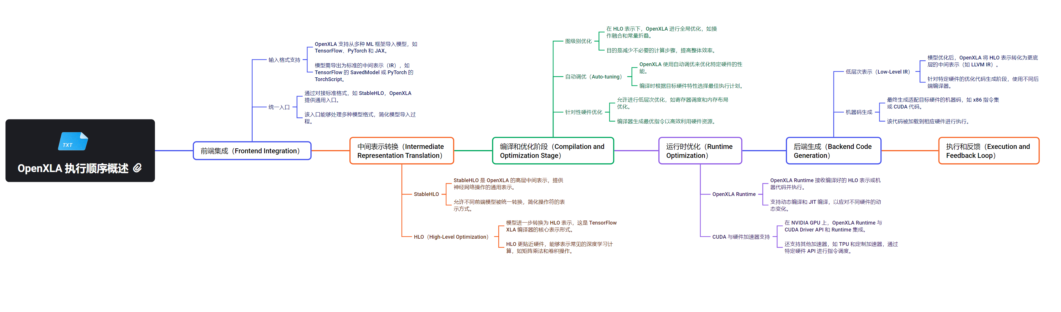
技术栈架构
1. 系统软件层
- CUDA Driver API:低级 API,提供对 NVIDIA GPU 的直接控制
- 允许直接管理设备、内存分配和程序执行
- 适用于需要细粒度控制的高级应用
- 为 OpenXLA 提供与 NVIDIA GPU 硬件交互的底层接口
2. 运行时环境层
- CUDA Runtime API:高级 API,简化了 GPU 编程,自动管理许多底层细节
- 为 OpenXLA 提供更高级的抽象,简化了 GPU 的使用
- 自动处理上下文管理和程序加载等任务
- OpenXLA Runtime:OpenXLA 框架的运行时环境
- 管理 OpenXLA 编译的模型的执行
- 支持多种硬件后端,包括 CUDA 设备
- 与 CUDA Runtime API 集成,提供对 NVIDIA GPU 的支持
3. 编程模型和语言层
- CUDA C/C++:扩展了 C/C++ 语言,允许开发者编写在 GPU 上运行的并行程序
- 为 OpenXLA 提供了一种与 NVIDIA GPU 交互的编程方式
- 可与 StableHLO 结合使用,实现对 CUDA 设备的优化
- StableHLO:OpenXLA 提供的高级中间表示语言
- 用于描述和优化机器学习模型
- 提供了一种声明式的方式来表达计算
- 可以针对 CUDA 设备等不同硬件后端进行优化
4. 计算库层
- NCCL:用于多 GPU 通信的库
- 支持多 GPU 之间的高效通信和数据交换
- 可与 OpenXLA 结合使用,支持分布式深度学习训练
5. 框架模型层
- PyTorch with OpenXLA:利用 OpenXLA 优化 PyTorch 模型在 CUDA 设备上的性能
- TensorFlow with OpenXLA:利用 OpenXLA 优化 TensorFlow 模型在 CUDA 设备上的性能
关系解析
OpenXLA 作为一个灵活的深度学习编译器框架,与 PyTorch 和 TensorFlow 深度集成,通过自定义算子、JIT 编译和 GPU 内核融合等技术,大幅提升了这些深度学习框架在 GPU 上的执行效率。同时,OpenXLA 还利用 CUDA Runtime API 和 CUDA Driver API,实现了对 GPU 硬件的精细控制和优化,包括内存管理、设备操作和内核启动等。这种多层次的架构设计使 OpenXLA 能够充分发挥 GPU 的计算能力,为开发者提供了一个高度灵活和易用的工具。此外,OpenXLA 还与 StableHLO 进行了深度集成,利用其提供的高级中间表示和优化技术,进一步增强了 OpenXLA 的性能和可扩展性。通过整合这些技术,OpenXLA 为开发者带来了显著的性能提升,同时简化了高性能深度学习应用的开发过程。
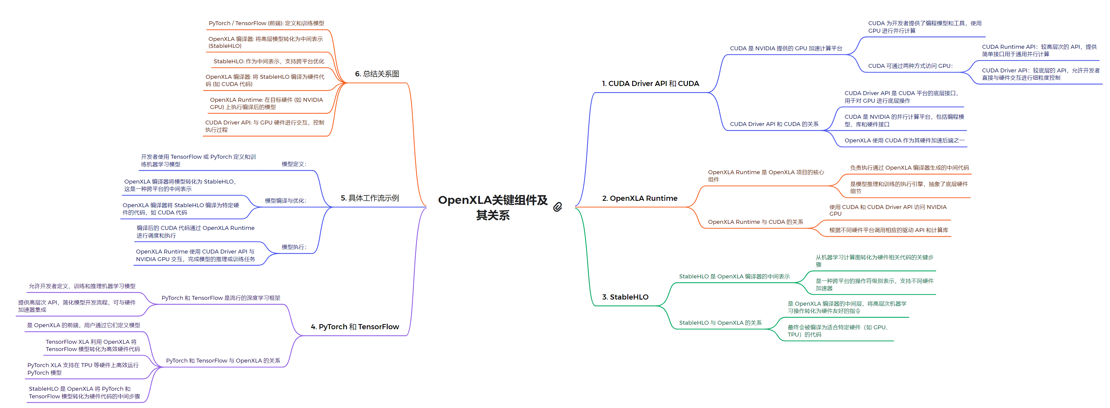
系统软件层
OpenXLA 通过使用 CUDA Driver API 与底层 GPU 进行交互,主要流程涉及从高层的模型执行到底层 GPU 资源的管理和调度:
-
OpenXLA 接收从 TensorFlow、PyTorch 等深度学习框架导出的模型(如 StableHLO 或 ONNX 格式)。
-
OpenXLA Runtime 解析模型,并通过图优化技术,减少冗余计算、调整执行顺序,以提升运行效率。
-
OpenXLA 会将优化后的模型图分解为多个子任务(操作),并对这些操作进行调度,分配给适合的硬件资源(如 CPU、GPU、TPU 等)。
-
通过 CUDA Driver API,OpenXLA 初始化 GPU 设备,包括检测可用的 GPU 设备、分配 GPU 资源等。
-
OpenXLA 通过 CUDA Driver API 请求 GPU 上的内存分配。使用
cuMemAlloc等 API 在 GPU 上分配全局内存。通过cuMemcpyHtoD(Host to Device)等 API 将 CPU 上的数据传输到 GPU 内存中。 -
OpenXLA 通过 CUDA Driver API 提交并启动计算核函数(Kernel),通常使用
cuLaunchKernel启动并行计算。 -
核函数会在 GPU 的并行计算单元(CUDA 核心)上运行,处理计算任务。
-
OpenXLA 负责为这些核函数设置执行配置(如网格大小、线程块大小等),确保高效并行执行。
-
在核函数执行结束后,OpenXLA 使用 CUDA Driver API 来同步执行流程,确保 GPU 的计算结果准备就绪,典型的 API 有
cuCtxSynchronize。 -
同时,OpenXLA 监控 GPU 执行的状态,处理可能的错误(如内存不足、非法访问等)。
-
通过
cuMemcpyDtoH(Device to Host)将 GPU 计算结果传回到 CPU 进行进一步处理。 -
完成计算后,OpenXLA 通过
cuMemFree等 API 释放在 GPU 上分配的内存资源。
运行时环境层
OpenXLA 可以通过底层库(例如 CUDA Runtime 或 CUDA Driver API)与 GPU 交互,但它不是直接用于设备查询或管理的工具。OpenXLA 的主要作用是为机器学习模型提供跨硬件的优化执行支持。OpenXLA 依赖于 CUDA API 进行设备信息查询。
- 定义了一个宏
CHECK_CUDA,用于检查 CUDA API 调用是否成功。如果失败,获取错误信息并退出程序。 - 调用
cuInit(0)初始化 CUDA 驱动程序。必须在所有 CUDA API 调用之前执行。 - 使用
cuDeviceGetCount(&deviceCount)获取系统中可用的 CUDA 设备数量,并打印出来。 - 使用
cuDeviceGet(&device, i)获取每个 CUDA 设备的句柄,用于后续查询设备信息。 - 使用
cuDeviceGetName(name, sizeof(name), device)获取每个设备的名称(例如 GPU 型号)。 - 使用
cuDeviceGetAttribute(&major, CU_DEVICE_ATTRIBUTE_COMPUTE_CAPABILITY_MAJOR, device)和cuDeviceGetAttribute(&minor, CU_DEVICE_ATTRIBUTE_COMPUTE_CAPABILITY_MINOR, device)获取设备的计算能力主版本和次版本。 - 使用
cuDeviceTotalMem(&totalMem, device)获取设备的总内存大小(以字节为单位),并转换为 MB 打印出来。
#include <stdio.h>
#include <cuda.h>

// CUDA 错误检查宏
#define CHECK_CUDA(call) do { \
    CUresult result = call; \
    if (result != CUDA_SUCCESS) { \
        const char *errStr; \
        cuGetErrorString(result, &errStr); \
        printf("CUDA Error: %s\n", errStr); \
        return -1; \
    } \
} while (0)

int main() {
    // 初始化 CUDA Driver API
    CHECK_CUDA(cuInit(0));

    // 获取设备数量
    int deviceCount = 0;
    CHECK_CUDA(cuDeviceGetCount(&deviceCount));

    printf("CUDA 设备数量: %d\n", deviceCount);

    // 遍历每个设备,获取设备信息
    for (int i = 0; i < deviceCount; ++i) {
        CUdevice device;
        char name[128];
        int major = 0, minor = 0;

        // 获取设备句柄
        CHECK_CUDA(cuDeviceGet(&device, i));

        // 获取设备名称
        CHECK_CUDA(cuDeviceGetName(name, sizeof(name), device));

        // 获取设备的计算能力 (Compute Capability)
        CHECK_CUDA(cuDeviceGetAttribute(&major, CU_DEVICE_ATTRIBUTE_COMPUTE_CAPABILITY_MAJOR, device));
        CHECK_CUDA(cuDeviceGetAttribute(&minor, CU_DEVICE_ATTRIBUTE_COMPUTE_CAPABILITY_MINOR, device));

        // 获取设备的总内存
        size_t totalMem = 0;
        CHECK_CUDA(cuDeviceTotalMem(&totalMem, device));

        printf("设备 %d: %s\n", i, name);
        printf("  计算能力: %d.%d\n", major, minor);
        printf("  总内存: %zu MB\n", totalMem / (1024 * 1024));
    }

    return 0;
}
结果:
CUDA 设备数量: 1
设备 0: NVIDIA GeForce RTX 4080 SUPER
  计算能力: 8.9
  总内存: 16072 MB
计算库层
在 XLA(Accelerated Linear Algebra)中使用自定义调用(Custom Call)机制,结合 XLA FFI(外部函数接口,Foreign Function Interface)来实现用户定义的操作。使用自定义调用在 CPU 上计算 A[i] = B[i % 128]+ C[i]。
xla::XlaBuilder:XLA 提供的用于构建计算图的类,这里实例化了一个名为 "do_it" 的构建器b。xla::Parameter:定义两个输入参数param0和param1。其中param0是一个长度为 128 的 1D 浮点型(F32)数组,param1是长度为 2048 的 1D 浮点型数组。xla::CustomCall:这是 XLA 中执行自定义操作的关键调用。通过传递"do_custom_call"字符串来指定自定义调用的名称,表示需要调用一个外部定义的函数。该自定义操作接收两个输入(param0和param1),输出结果的形状是一个长度为 2048 的 F32 数组。BufferF32:这是 XLA FFI 中的类型别名,表示一个 1D 的浮点型(F32)缓冲区。- in0
和in1是输入缓冲区(分别为 param0 和 param1 的数据),它们的数据类型为BufferF32out是输出缓冲区,存储结果。该函数的逻辑为:将in0和in1中的数据进行逐元素相加,并将结果写入输出缓冲区。注意这里通过i % d0来处理in0,使得其在计算时按顺序重复。assert检查输出缓冲区的维度,确保与in1的维度相同。 - 定义了一个处理器
handler,并将它绑定到do_custom_call函数上。通过这种绑定,FFI 可以知道自定义调用应该如何匹配到 C++ 函数。绑定过程中明确指定了函数的参数类型和返回值类型为Buffer(即 1D 缓冲区)。 - 将处理器
handler注册到 XLA FFI,表示它将在 "Host" 平台上可用。 "do_custom_call"是自定义调用的名称,与xla::CustomCall中使用的名称一致。xla::ffi::GetXlaFfiApi()获取当前的 XLA FFI API 实例,确保处理器能够正确注册到 XLA。
#include "xla/client/xla_builder.h"
#include "xla/service/custom_call_target_registry.h"

void do_it() {
  xla::XlaBuilder b("do_it");
  xla::XlaOp param0 =
      xla::Parameter(&b, 0, xla::ShapeUtil::MakeShape(xla::F32, {128}), "p0");
  xla::XlaOp param1 =
      xla::Parameter(&b, 1, xla::ShapeUtil::MakeShape(xla::F32, {2048}), "p1");
  xla::XlaOp custom_call =
      xla::CustomCall(&b, "do_custom_call", /*operands=*/{param0, param1},
        /*shape=*/xla::ShapeUtil::MakeShape(xla::F32, {2048}),
        /*opaque=*/"", /*has_side_effect=*/false,
        /*output_operand_aliasing=*/{}, /*literal=*/nullptr,
        /*schedule=*/CustomCallSchedule::SCHEDULE_NONE,
        /*api_version=*/CustomCallApiVersion::API_VERSION_TYPED_FFI);
}

// Constrain custom call arguments to rank-1 buffers of F32 data type.
using BufferF32 = xla::ffi::BufferR1<xla::ffi::DataType::F32>;

// Implement a custom call as a C+ function. Note that we can use `Buffer` type
// defined by XLA FFI that gives us access to buffer data type and shape.
xla::ffi::Error do_custom_call(BufferF32 in0, BufferF32 in1,
                               xla::ffi::Result<BufferF32> out) {
  size_t d0 = in0.dimensions[0];
  size_t d1 = in1.dimensions[0];

  // Check that dimensions are compatible.
  assert(out->dimensions[0] == d1 && "unexpected dimensions");

  for (size_t i = 0; i < d1; ++i) {
    out->data[i] = in0.data[i % d0] + in1.data[i];
  }
}

// Explicitly define an XLA FFI handler signature and bind it to the
// `do_custom_call` implementation. XLA FFI handler can automatically infer
// type signature from the custom call function, but it relies on magical
// template metaprogramming an explicit binding provides and extra level of
// type checking and clearly states custom call author intentions.
XLA_FFI_DEFINE_HANDLER(handler, do_custom_call,
                       ffi::Ffi::Bind()
                           .Arg<Buffer>()
                           .Arg<Buffer>()
                           .Ret<Buffer>());

// Registers `handler` with and XLA FFI on a "Host" platform.
XLA_FFI_REGISTER_HANDLER(xla::ffi::GetXlaFfiApi(), "do_custom_call",
                         "Host", handler);
在原有的 XLA 的自定义调用实现上进行了扩展,增加了 GPU 加速部分,主要通过 CUDA 来并行处理自定义操作的逻辑,计算 A[i] = B[i % 128] + C[i]。
- 构建了 XLA 的计算图,通过
xla::CustomCall调用了名为"do_custom_call"的自定义操作。它定义了两个输入参数param0和param1,并设置输出为长度为 2048 的浮点数数组。 const float* in0, const float* in1, float* out:输入in0和in1是常量浮点型数组指针,out是输出数组指针。size_t idx = blockIdx.x * blockDim.x + threadIdx.x:计算当前线程的全局索引idx。blockIdx.x是当前线程块的索引,blockDim.x是每个线程块的大小,threadIdx.x是当前线程在块内的索引。out[idx] = in0[idx % 128] + in1[idx]:对于每个线程,执行in0[idx % 128] + in1[idx],并将结果写入out[idx]。in0的大小为 128,因此使用% 128使得in0的数据循环重复使用,而in1和out都是长度为 2048。block_dim和grid_dim:用于定义 CUDA kernel 的执行配置。block_dim设置为 64,表示每个线程块中有 64 个线程,grid_dim设置为2048 / 64,即 32 个线程块。每个线程块并行处理 64 个数据元素,共 2048 个数据元素。custom_call_kernel<<<grid_dim, block_dim, 0, stream>>>(in0.data, in1.data, out->data):通过 CUDA 启动custom_call_kernel内核,传入输入和输出数据指针,以及 CUDA 流stream,让 GPU 并行执行数据计算。XLA_FFI_DEFINE_HANDLER:定义一个新的 XLA FFI 处理器handler,并将其绑定到do_custom_call函数。.Ctx<xla::ffi::PlatformStream<CUstream>>():这行代码表明do_custom_call函数需要接受一个 CUDA 流CUstream作为上下文,以便在 GPU 上执行自定义调用。.Arg<BufferF32>():定义两个参数,类型为BufferF32(浮点数组)。.Ret<BufferF32>():定义返回值为BufferF32。XLA_FFI_REGISTER_HANDLER:将定义好的handler注册到 XLA FFI 中,使得 XLA 可以识别并调用这个自定义操作。
void do_it() { /* same implementation as above */ }

__global__ custom_call_kernel(const float* in0, const float* in1, float* out) {
  size_t idx = blockIdx.x * blockDim.x + threadIdx.x;
  out[idx] = in0[idx % 128] + in1[idx];
}

void do_custom_call(CUstream stream, BufferF32 in0, BufferF32 in1,
                    xla::ffi::Result<BufferF32> out) {
  size_t d0 = in0.dimensions[0];
  size_t d1 = in1.dimensions[0];
  size_t d2 = out->dimensions[0];

  assert(d0 == 128 && d1 == 2048 && d2 == 2048 && "unexpected dimensions");

  const int64_t block_dim = 64;
  const int64_t grid_dim = 2048 / block_dim;
  custom_call_kernel<<<grid_dim, block_dim, 0, stream>>>(
    in0.data, in1.data, out->data);
}

XLA_FFI_DEFINE_HANDLER(handler, do_custom_call,
                       ffi::Ffi::Bind()
                           .Ctx<xla::ffi::PlatformStream<CUstream>>()
                           .Arg<BufferF32>()
                           .Arg<BufferF32>()
                           .Ret<BufferF32>());

XLA_FFI_REGISTER_HANDLER(xla::ffi::GetXlaFfiApi(), "do_custom_call",
                         "CUDA", handler);
为 TensorFlow 启用 XLA,使用@tf.function(jit_compile=True)进行显式编译,显式编译 API 提供精细的控制,用于选择应编译哪些函数。例如,以下执行 MNIST 训练的 TensorFlow 函数使用 XLA 进行编译:
@tf.function(jit_compile=True)
def train_mnist(images, labels):
    images, labels = cast(images, labels)

    with tf.GradientTape() as tape:
      predicted_labels = layer(images)
      loss = tf.reduce_mean(tf.nn.sparse_softmax_cross_entropy_with_logits(
          logits=predicted_labels, labels=labels
      ))
    layer_variables = layer.trainable_variables
    grads = tape.gradient(loss, layer_variables)
    optimizer.apply_gradients(zip(grads, layer_variables))
tfcompile 是 XLA编译器工具,可以将 TensorFlow 图进行提前(AOT)编译,生成可执行代码。它有助于减少二进制文件的整体大小,并能避免部分运行时开销。tfcompile 接收一个子图(通过 TensorFlow 的 Feed 和 Fetch 概念定义),并生成实现该子图的函数。Feed 对应函数的输入参数,Fetch 对应函数的输出参数。所有输入必须通过 Feed 完全指定,生成的子图不能包含占位符或变量节点。通常的做法是将所有占位符和变量标记为 Feed,以确保最终生成的子图中没有这些节点。
使用 tfcompile 编译 TensorFlow 子图,首先,需要定义一个简单的 TensorFlow 模型或子图。以下是一个定义子图的示例,输入为标量,输出为其平方。
import tensorflow as tf

# 创建计算图
def simple_graph(x):
    return tf.math.square(x)

# 输入符号化
x = tf.placeholder(dtype=tf.float32, shape=(), name='input')

# 定义子图
y = simple_graph(x)

# 将计算图保存到文件
with tf.Session() as sess:
    tf.io.write_graph(sess.graph_def, './', 'simple_graph.pbtxt')
tfcompile 需要一个配置文件,指定输入、输出及其他信息。配置文件 config.pbtxt 示例:
# config.pbtxt
feed {
  id { node_name: "input" }
  shape { dim { size: 1 } }  # 指定输入张量的形状
}
fetch {
  id { node_name: "Square" }  # 这是子图输出节点的名称
}
使用 tfcompile 编译器编译生成可执行二进制文件。生成的 .o 文件还需要链接到可执行程序。下面是 C++ 示例,展示如何使用生成的二进制文件:
#include <iostream>
#include "compiled_graph.o"

int main() {
    // 创建输入张量
    MyCompiledGraph computation;
    float input_value = 3.0;
    float output_value;

    // 执行计算
    computation.compute(&input_value, &output_value);

    std::cout << "输入值: " << input_value << " 的平方是: " << output_value << std::endl;
    return 0;
}
编译运行后输出如下内容:
输入值: 3 的平方是: 9
为 pytorch启用 XLA,PyTorch/XLA 使用与常规 PyTorch 相同的接口,但有一些附加功能。导入会torch_xla初始化 PyTorch/XLA,并 xm.xla_device()返回当前 XLA 设备。
import torch
import torch_xla
import torch_xla.core.xla_model as xm

t = torch.randn(2, 2, device=xm.xla_device())
print(t.device)
print(t)
结果
xla:0
tensor([[ 0.1028, -1.4783],
        [-0.4271,  1.3415]], device='xla:0')
与其他设备类型一样,XLA 张量仅与同一设备上的其他 XLA 张量配合使用。
l_in = torch.randn(10, device=xm.xla_device())
linear = torch.nn.Linear(10, 20)
l_out = linear(l_in)
print(l_out)
# Input tensor is not an XLA tensor: torch.FloatTensor
张量从 CPU 移动到 XLA 设备:当张量从 CPU 移动到 XLA 设备(如 TPU、GPU)时,数据会被复制到目标设备的内存中。这意味着可以在加速硬件上执行计算。同样,XLA 设备上的张量可以移动回 CPU,在这个过程中,数据会从设备复制回 CPU 的内存。一旦张量数据被复制到另一台设备,两个设备上的张量副本之间不会有任何联系。每个副本在各自的设备内存中独立存在。
应在保存之前将 XLA 张量移至 CPU,如以下代码片段所示:
import torch
import torch_xla
import torch_xla.core.xla_model as xm

device = xm.xla_device()

t0 = torch.randn(2, 2, device=device)
t1 = torch.randn(2, 2, device=device)

tensors = (t0.cpu(), t1.cpu())

torch.save(tensors, 'tensors.pt')

tensors = torch.load('tensors.pt')

t0 = tensors[0].to(device)
t1 = tensors[1].to(device)
print(t0)
print(t1)
结果
tensor([[ 0.1028, -1.4783],
        [-0.4271,  1.3415]], device='xla:0')
tensor([[ 0.8257,  0.3266],
        [ 0.9146, -0.2747]], device='xla:0')
框架模型层
使用了 PyTorch XLA 来在 XLA(如 TPU 等加速设备)上运行张量操作。
-
引入
torch、torch_xla和torch_xla.core.xla_model,用于在 XLA 设备上执行 PyTorch 操作。 -
使用
torch.randn(2, 2, device=xm.xla_device())创建一个 2x2 的随机张量t,并将其分配到 XLA 设备。 -
创建两个 2x2 的随机张量
t0和t1,并进行逐元素加法和矩阵乘法,打印结果。 -
创建一个大小为 10 的随机输入向量
l_in,并将其分配到 XLA 设备。 -
定义一个输入特征为 10、输出特征为 20 的线性层
linear,并迁移到 XLA 设备。 -
将输入
l_in传入线性层,得到输出l_out,并打印输出结果。
import torch
import torch_xla
import torch_xla.core.xla_model as xm

t = torch.randn(2, 2, device=xm.xla_device())
print(t.device)
print(t)

t0 = torch.randn(2, 2, device=xm.xla_device())
t1 = torch.randn(2, 2, device=xm.xla_device())
print(t0 + t1)
print(t0.mm(t1))

#神经网络
l_in = torch.randn(10, device=xm.xla_device())
linear = torch.nn.Linear(10, 20).to(xm.xla_device())
l_out = linear(l_in)
print(l_out)
结果
xla:0
tensor([[ 0.1028, -1.4783],
        [-0.4271,  1.3415]], device='xla:0')
tensor([[ 1.7679,  0.2210],
        [ 0.5831, -1.5733]], device='xla:0')
tensor([[ 0.6698, -0.5113],
        [ 0.9527,  0.2601]], device='xla:0')
tensor([-0.8333,  0.4356,  0.4277, -0.3944,  0.8075,  0.3516,  0.0455,  0.0778,
        -0.0822,  0.4418, -0.7217,  0.3582, -0.7285,  0.1117, -0.0466, -0.7045,
        -0.1443,  0.3461, -0.3151, -0.6094], device='xla:0',
       grad_fn=<AddBackward0>)
实现了一个使用 PyTorch XLA 再 TPU 训练和评估 MNIST 手写数字分类模型的完整流程,包括数据加载、模型构建、训练、保存和推理。
- 引入所需的 PyTorch 和 Torch XLA 库,以及 MNIST 数据集和数据处理工具。设置设备为 TPU,使用
xm.xla_device()。 - 使用
transforms.Compose创建数据转换,将 MNIST 数据集中的图像转换为张量。下载 MNIST 训练集并创建数据加载器train_loader,设置批量大小为 64,并随机打乱数据。 - 定义一个简单的神经网络模型,包括:扁平化层,将 28x28 的图像展平成一维。128 单元的全连接层,使用 ReLU 激活函数。10 单元的全连接层,使用 LogSoftmax 激活函数。将模型迁移到 TPU 设备。
- 使用负对数似然损失函数
NLLLoss。使用随机梯度下降优化器SGD,学习率为 0.01,动量为 0.9。 - 对训练数据进行迭代:清零优化器的梯度。将数据和目标迁移到 TPU 设备。通过模型进行前向传播,计算损失。进行反向传播以计算梯度。更新模型参数。调用
xm.mark_step()同步 TPU。 - 使用
torch.save()保存训练好的模型到mnist_model_full.pth文件中。 - 加载保存的模型,并将其迁移到 TPU 设备,切换到评估模式。
- 在不计算梯度的上下文中:遍历测试数据,迁移到 TPU 设备。进行前向传播,计算输出。使用
torch.max()获取预测结果的最大值索引。打印预测结果,且仅处理一个批次作为示例。
import torch
import torch.nn as nn
import torch.optim as optim
import torch_xla.core.xla_model as xm
from torch.utils.data import DataLoader
from torchvision.datasets import MNIST
from torchvision import transforms

# 设备设定(TPU)
device = xm.xla_device()

# 数据集与数据加载器设定
transform = transforms.Compose([transforms.ToTensor()])
train_dataset = MNIST(root='data', train=True, transform=transform, download=True)
train_loader = DataLoader(train_dataset, batch_size=64, shuffle=True)

# 模型设定
model = nn.Sequential(
    nn.Flatten(),
    nn.Linear(28*28, 128),
    nn.ReLU(),
    nn.Linear(128, 10),
    nn.LogSoftmax(dim=1)
).to(device)

# 损失函数和优化器设定
loss_fn = nn.NLLLoss()
optimizer = optim.SGD(model.parameters(), lr=0.01, momentum=0.9)

# 训练循环
for data, target in train_loader:
    optimizer.zero_grad()
    data = data.to(device)
    target = target.to(device)
    output = model(data)
    loss = loss_fn(output, target)
    loss.backward()

    optimizer.step()
    xm.mark_step()  # TPU同步

# 保存整个模型
torch.save(model, 'mnist_model_full.pth')

# 模型推理
import torch

# 加载整个模型
model = torch.load('mnist_model_full.pth').to(device)
model.eval()  # 切换到评估模式

# 加载测试数据
test_dataset = MNIST(root='data', train=False, transform=transform, download=True)
test_loader = DataLoader(test_dataset, batch_size=64, shuffle=False)

# 使用模型进行推理
with torch.no_grad():  # 禁用梯度计算以加快推理
    for data, _ in test_loader:
        data = data.to(device)
        output = model(data)
        xm.mark_step()  # TPU同步

        # 获取预测结果
        _, predicted = torch.max(output, 1)
        print(predicted)
        break  # 仅处理一个批次的示例
结果
tensor([7, 2, 1, 0, 4, 1, 4, 9, 6, 9, 0, 6, 9, 0, 1, 5, 9, 7, 3, 4, 9, 6, 6, 5,
        4, 0, 7, 4, 0, 1, 3, 1, 3, 6, 7, 2, 7, 1, 2, 1, 1, 7, 4, 2, 3, 5, 1, 2,
        4, 4, 6, 3, 5, 5, 6, 0, 4, 1, 9, 5, 7, 8, 4, 3], device='xla:0')
将一个 PyTorch 模型导出并转换为一种适合跨平台应用的格式( StableHLO ),以便进行优化、部署和进一步分析。
- 模型加载:加载了预训练的 ResNet-18 模型,使用
torchvision提供的默认权重。 - 样本输入生成:创建了一个形状为
(4, 3, 224, 224)的随机张量,模拟输入的图像数据。 - 模型导出:使用
export函数将 ResNet-18 模型导出为中间表示,以便后续处理。 - 转换为 StableHLO:将导出的模型转换为 StableHLO 格式,适用于跨平台优化和部署。
- 输出 StableHLO 文本:打印模型前向计算图的 StableHLO 文本表示的前 400 个字符,以供检查和分析。
import torch
import torchvision
from torch.export import export

resnet18 = torchvision.models.resnet18(weights=torchvision.models.ResNet18_Weights.DEFAULT)
sample_input = (torch.randn(4, 3, 224, 224), )
exported = export(resnet18, sample_input)

from torch_xla.stablehlo import exported_program_to_stablehlo

stablehlo_program = exported_program_to_stablehlo(exported)
print(stablehlo_program.get_stablehlo_text('forward')[0:400],"\n...")
结果
module @IrToHlo.484 attributes {mhlo.cross_program_prefetches = [], mhlo.is_dynamic = false, mhlo.use_auto_spmd_partitioning = false} {
  func.func @main(%arg0: tensor<1000xf32>, %arg1: tensor<1000x512xf32>, %arg2: tensor<512xf32>, %arg3: tensor<512xf32>, %arg4: tensor<512xf32>, %arg5: tensor<512xf32>, %arg6: tensor<512x256x1x1xf32>, %arg7: tensor<256xf32>, %arg8: tensor<256xf32>, %arg9: tensor<25
...
- 定义一个简单的加法模型,并创建输入数据。
- 将模型导出为中间表示,并转换为 StableHLO 格式,便于跨平台应用和优化。
- 最后,输出转换后的模型信息,便于分析和调试。
import torch
import torch.nn as nn
from torch.export import export
from torch_xla.stablehlo import exported_program_to_stablehlo

# 定义一个简单的加法模型
class AddModel(nn.Module):
    def __init__(self):
        super(AddModel, self).__init__()

    def forward(self, x, y):
        return x + y

# 创建模型实例
add_model = AddModel()

# 创建示例输入
x_input = torch.randn(4, 3, 224, 224)  # 第一个输入
y_input = torch.randn(4, 3, 224, 224)  # 第二个输入

# 使用 export 函数导出模型
exported = export(add_model, (x_input, y_input))

# 将导出的模型转换为 StableHLO 格式
stablehlo_program = exported_program_to_stablehlo(exported)

# 打印 StableHLO 程序文本的一部分
print(stablehlo_program.get_stablehlo_text('forward')[0:400], "\n...")
结果
module @IrToHlo.8 attributes {mhlo.cross_program_prefetches = [], mhlo.is_dynamic = false, mhlo.use_auto_spmd_partitioning = false} {
  func.func @main(%arg0: tensor<4x3x224x224xf32>, %arg1: tensor<4x3x224x224xf32>) -> tensor<4x3x224x224xf32> {
    %0 = stablehlo.add %arg1, %arg0 : tensor<4x3x224x224xf32>
    return %0 : tensor<4x3x224x224xf32>
  }
}
实现了使用 TensorFlow 定义一个简单的神经网络模型,生成随机输入,并使用 XLA(加速线性代数)优化进行前向传播。
- 使用
tf.config.list_physical_devices('GPU')检查可用的 GPU 数量。输出可用 GPU 的数量。 - 使用
tf.keras.Sequential创建一个顺序模型。第一层是一个全连接层(Dense),有 10 个单元,输入维度为 10,激活函数为 ReLU。第二层是另一个全连接层,包含 5 个单元,激活函数为 softmax。 - 定义批量大小(
batch_size)为 16,输入向量维度(input_vector_dim)为 10。使用tf.random.normal生成形状为(16, 10)的随机输入。 - 使用
@tf.function(jit_compile=True)装饰器定义前向传播函数,以启用 XLA 优化。函数接受输入并返回模型的输出。 - 调用前向传播函数
forward_pass,传入随机输入进行计算。
import tensorflow as tf

print("Num GPUs Available: ", len(tf.config.list_physical_devices('GPU')))

# Define the model
model = tf.keras.Sequential(
    [tf.keras.layers.Dense(10, input_shape=(10,), activation="relu"),
     tf.keras.layers.Dense(5, activation="softmax")]
)

# Generate random inputs for the model
batch_size = 16
input_vector_dim = 10
random_inputs = tf.random.normal((batch_size, input_vector_dim))

# Run a forward pass
_ = model(random_inputs)

# Compile the model function with XLA optimization
@tf.function(jit_compile=True)
def forward_pass(inputs):
    return model(inputs)

# Run the forward pass with XLA
_ = forward_pass(random_inputs)
结果
I0000 00:00:1727407770.382644 1007512 service.cc:146] XLA service 0x8ec22c0 initialized for platform CUDA (this does not guarantee that XLA will be used). Devices:
I0000 00:00:1727407770.382662 1007512 service.cc:154]   StreamExecutor device (0): NVIDIA GeForce RTX 4080 SUPER, Compute Capability 8.9
2024-09-27 11:29:30.387574: I tensorflow/compiler/mlir/tensorflow/utils/dump_mlir_util.cc:268] disabling MLIR crash reproducer, set env var `MLIR_CRASH_REPRODUCER_DIRECTORY` to enable.
2024-09-27 11:29:31.040309: I external/local_xla/xla/stream_executor/cuda/cuda_dnn.cc:531] Loaded cuDNN version 8907
I0000 00:00:1727407771.151882 1007512 device_compiler.h:188] Compiled cluster using XLA!  This line is logged at most once for the lifetime of the process.
OpenACC
OpenACC 是一种用于异构计算系统(如 GPU 加速器)的编程模型,它允许程序员通过指令简化代码的并行化和加速。它的技术栈可以分为几个层次,从底层硬件到高层的应用框架,包括系统软件层、运行时环境层、编程模型和语言层、计算库层和框架模型层。
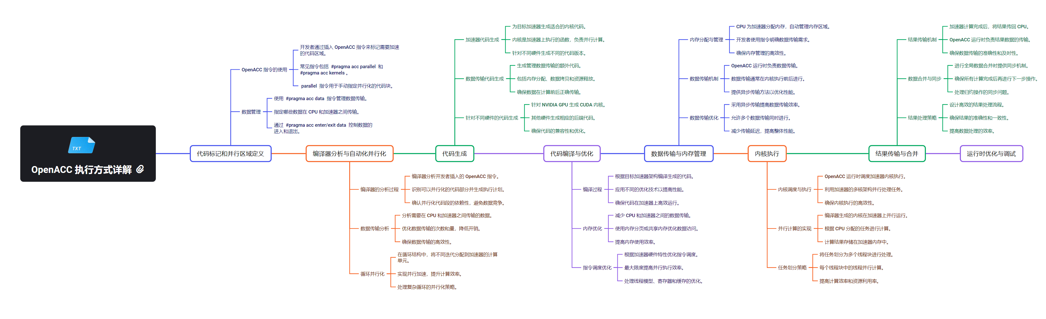
OpenACC作为一种异构并行编程标准,通过指指令集的方式,为开发者提供了一种简单高效的方法来利用GPU等加速器进行并行计算。从图中可以看到,OpenACC与CUDA Runtime API和CUDA Driver API存在密切联系,利用这些底层API实现了对GPU硬件的精细控制和优化,包括内存管理、设备操作和内核启动等。同时,OpenACC还与编程语言和编译器技术深度集成,如支持C/C++和Fortran,并与OpenMP、OpenCL等其他并行编程模型进行了融合,形成了一个丰富的异构计算生态系统。这种多层次的架构设计使OpenACC能够充分发挥GPU的计算能力,为开发者带来显著的性能提升,同时简化了高性能应用的开发过程。
技术栈架构
技术栈架构
1. 系统软件层
- 驱动程序(Driver):如 CUDA 驱动(针对 NVIDIA GPU)或 ROCm 驱动(针对 AMD GPU),这些驱动为硬件提供低级访问接口,并支持高层编程模型(如 OpenACC)与硬件之间的通信。
2. 运行时环境层
- OpenACC Runtime Library:OpenACC 运行时库支持运行时系统的指令调度和执行。它负责管理并行任务的启动、内存分配、主机与设备之间的数据传输等工作。
- CUDA/ROCm Runtime:如果 OpenACC 程序运行在 NVIDIA 或 AMD GPU 上,实际的并行执行由底层 CUDA 或 ROCm 运行时环境完成。
3. 编程模型和语言层
- OpenACC 规范:OpenACC 使用编译指令(directives)的方式对现有代码进行注释,指示编译器如何并行化和加速代码。指令以
#pragma acc开始,附带对并行执行、循环分配、数据传输等操作的具体说明。 - C/C++ 和 Fortran:OpenACC 编译指令可以与标准的 C/C++ 和 Fortran 语言配合使用,便于将现有代码改造为并行化代码。
4. 计算库层
- cuBLAS、cuFFT(针对 NVIDIA):这些库为线性代数、傅里叶变换等常用计算提供高效实现,可以在 OpenACC 应用中被调用,从而减少手动编写复杂并行代码的需求。
- rocBLAS、rocFFT(针对 AMD):这是 AMD 提供的类似库,支持基于 ROCm 的加速计算。
5. 框架模型层
- 数值模拟和科学计算框架:如 LAMMPS、GROMACS、ANSYS 等,它们在模拟大规模物理现象(如分子动力学、流体力学)时可以通过 OpenACC 加速特定的计算模块。
- 深度学习框架:尽管 OpenACC 本身不是主流的深度学习加速技术,但某些框架可以通过集成 OpenACC 指令优化特定的计算内核。
- HPC 应用框架:如 OpenFOAM 和 WRF,这些高性能计算应用框架可以通过 OpenACC 进行并行化,以提高在多核和异构环境中的执行效率。
关系解析
 OpenACC作为一种异构并行编程标准,通过指令集的方式为开发者提供了一种简单高效的方法来利用GPU进行并行计算。从图中可以看到,OpenACC与CUDA Runtime API和CUDA Driver API存在密切联系,利用这些底层API实现了对GPU硬件的精细控制和优化,包括内存管理、设备操作和内核启动等。同时,OpenACC还与编程语言和编译器技术深度集成,如支持C/C++和Fortran,并与OpenMP、OpenCL等其他并行编程模型进行了融合,形成了一个丰富的异构计算生态系统。此外,OpenACC还与NVIDIA特定的技术,如NCCL、Tensor Cores等进行了深度集成,进一步提升了在NVIDIA GPU上的性能和优化。这种多层次的架构设计使OpenACC能够充分发挥GPU的计算能力,为开发者带来显著的性能提升,同时简化了高性能应用的开发过程。
系统软件层
OpenACC 是一种用于异构计算系统(如 GPU 加速器)的编程模型,它允许程序员通过指令简化代码的并行化和加速。
OpenACC 编译器会将程序转换为包含并行指令的代码,而运行时环境层则负责管理这些指令的执行,包括内存管理、数据移动和调度。
- OpenACC Runtime Library:OpenACC 运行时库支持运行时系统的指令调度和执行。它负责管理并行任务的启动、内存分配、主机与设备之间的数据传输等工作。
- CUDA/ROCm Runtime:如果 OpenACC 程序运行在 NVIDIA 或 AMD GPU 上,实际的并行执行由底层 CUDA 或 ROCm 运行时环境完成。
这是 OpenACC 核心的层次,程序员使用 OpenACC 的编程模型和语言构建并行程序。
- OpenACC 规范:OpenACC 使用编译指令(directives)的方式对现有代码进行注释,指示编译器如何并行化和加速代码。指令以
#pragma acc开始,附带对并行执行、循环分配、数据传输等操作的具体说明。 - C/C++ 和 Fortran:OpenACC 编译指令可以与标准的 C/C++ 和 Fortran 语言配合使用,便于将现有代码改造为并行化代码。
为了进一步提升性能和开发效率,OpenACC 编程环境下也可以使用许多预构建的高性能计算库。
- cuBLAS、cuFFT(针对 NVIDIA):这些库为线性代数、傅里叶变换等常用计算提供高效实现,可以在 OpenACC 应用中被调用,从而减少手动编写复杂并行代码的需求。
- rocBLAS、rocFFT(针对 AMD):这是 AMD 提供的类似库,支持基于 ROCm 的加速计算。
- OpenACC 兼容的第三方库:一些第三方库可以与 OpenACC 代码集成,处理专门的计算需求。
在高层应用中,用户通常使用现成的计算框架,它们可以通过 OpenACC 进行优化以加速大规模计算任务。
- 数值模拟和科学计算框架:如 LAMMPS、GROMACS、ANSYS 等,它们在模拟大规模物理现象(如分子动力学、流体力学)时可以通过 OpenACC 加速特定的计算模块。
- 深度学习框架:尽管 OpenACC 本身不是主流的深度学习加速技术,但某些框架可以通过集成 OpenACC 指令优化特定的计算内核。
- HPC 应用框架:如 OpenFOAM 和 WRF,这些高性能计算应用框架可以通过 OpenACC 进行并行化,以提高在多核和异构环境中的执行效率。
OpenACC 使用 CUDA Driver API 与底层 GPU 进行交互的流程可以分为几个关键步骤:
-
OpenACC 程序通过编译器(如
PGI或GCC)编译,这些编译器支持将 OpenACC 指令转换为 CUDA 代码。编译器生成的代码中包含针对 GPU 的 CUDA 内核,并通过 CUDA Driver API 与 GPU 进行通信和管理。 -
程序开始时,CUDA Driver API 初始化 CUDA 设备。具体流程为:调用
cuInit()函数,初始化 CUDA 驱动。使用cuDeviceGet()函数选择目标 GPU 设备。使用cuCtxCreate()创建一个与 GPU 设备关联的上下文(Context),用于后续的操作。 -
使用
cuMemAlloc()函数在 GPU 设备上分配内存。使用cuMemcpyHtoD()将主机(CPU)上的数据传输到设备(GPU)。执行计算完成后,使用cuMemcpyDtoH()将结果从设备传回主机。 -
OpenACC 编译器将 OpenACC 代码中的并行指令转换为 CUDA 内核,调用 CUDA Driver API 的
cuLaunchKernel()函数启动内核执行。 -
CUDA Driver API 提供了错误检查机制,可以通过
cuGetErrorName()和cuGetErrorString()函数获取错误信息。 -
当计算完成后,使用
cuMemFree()释放在 GPU 上分配的内存。 -
最后,调用
cuCtxDestroy()销毁与 GPU 关联的上下文,释放资源。
运行时环境层
实现了使用 OpenACC 和 CUDA Runtime API 的 C 程序,用于获取和打印 CUDA 设备的信息。
这段代码的主要功能和要点如下:
- CUDA 设备数量获取:通过
acc_get_num_devices获取系统中可用的 NVIDIA CUDA 设备数量,并打印出来。 - 设备属性查询:循环遍历每个设备,使用
cudaGetDeviceProperties获取设备名称、计算能力和全局内存大小。 - 错误处理:使用
cudaCheckError宏简化了对 CUDA 函数调用的错误检查。 - CUDA 驱动版本获取:通过
cudaDriverGetVersion获取当前 CUDA 驱动的版本信息并打印。
#include <stdio.h>
#include <openacc.h>
#include <cuda_runtime.h>

// CUDA 错误检查宏
#define cudaCheckError(call)                                                    \
    {                                                                           \
        cudaError_t cudaStatus = call;                                          \
        if (cudaStatus != cudaSuccess) {                                        \
            fprintf(stderr, "CUDA Error: %s at line %d\n",                      \
                    cudaGetErrorString(cudaStatus), __LINE__);                  \
            exit(cudaStatus);                                                   \
        }                                                                       \
    }

int main() {
    int num_devices = acc_get_num_devices(acc_device_nvidia);
    printf("Total CUDA devices found: %d\n", num_devices);

    for (int device_id = 0; device_id < num_devices; device_id++) {
        acc_set_device_num(device_id, acc_device_nvidia);

        // 使用 CUDA Runtime API 获取设备信息
        cudaDeviceProp deviceProp;
        cudaCheckError(cudaGetDeviceProperties(&deviceProp, device_id));

        printf("\nDevice %d: %s\n", device_id, deviceProp.name);
        printf("  Compute capability: %d.%d\n", deviceProp.major, deviceProp.minor);
        printf("  Total global memory: %.2f GB\n", (float)deviceProp.totalGlobalMem / (1024 * 1024 * 1024));
    }

    // 获取 CUDA 驱动版本
    int driver_version = 0;
    cudaCheckError(cudaDriverGetVersion(&driver_version));
    printf("\nCUDA Driver version: %d\n", driver_version / 1000);

    return 0;
}
结果:
Total CUDA devices found: 1

Device 0: NVIDIA GeForce RTX 4080 SUPER
  Compute capability: 8.9
  Total global memory: 15.70 GB

CUDA Driver version: 12
编程模型和语言层
下面这段代码主要演示了如何使用 OpenACC 在并行环境中安全地对数组进行多种操作,实现了对一个数组进行并行处理,主要功能包括读取、写入、捕获和更新操作。并通过原子操作防止数据竞争。
-
创建并初始化一个大小为 100 的数组
data,内容为 0 到 99。 -
在并行环境中,检查数组元素值是否大于等于 50,若是,则将该元素的索引值赋给
readSum。 -
在并行环境中,检查数组元素值是否大于等于 50,若是,则计算
x * 2 + 1并将其赋值给writeSum。 -
在并行环境中,检查数组元素值是否大于等于 50,若是,则将该元素的值赋给
captureSum,并将该元素自减 1(减少其值)。 -
在并行环境中,检查数组元素值是否大于等于 50,若是,则对
updateSum进行自增操作,计算符合条件的元素个数。 -
最后输出
captureSum的值,这个值是从数组中捕获的元素值,并在捕获后减少了对应的元素。
#include "iostream"
#include "stdlib.h"

int main(){
    int n = 100;
    double * data = (double *)malloc( n * sizeof(double));
    for( int x = 0; x < n; ++x){
	    data[x] = x;
    }

    double readSum = 0.0;
    double writeSum = 0.0;
    double captureSum = 0.0;
    double updateSum = 0.0;

    // the atomic construct prevents reading the value while a gang/worker/vector is writing and vice versa
    // this is the read clause read the value of one variable into another variable
    #pragma acc parallel loop copy(data[0:n]) copyout(readSum)
    for(int x = 0; x < n; ++x){
        if(data[x] >= n/2){
            #pragma acc atomic read
            readSum = x;
        }
    }

    // the atomic construct prevents reading the value while a gang/worker/vector is writing and vice versa
    // this is the write clause that only allows a direct write to a variable from a expression
    #pragma acc parallel loop copy(data[0:n]) copyout(writeSum)
    for(int x = 0; x < n; ++x){
        if(data[x] >= n/2){
            #pragma acc atomic write
            writeSum = x*2 + 1;
        }
    }

    //this is the capture clause that the update to the expression into another variable
    #pragma acc parallel loop copy(data[0:n]) copyout(captureSum)
    for(int x = 0; x < n; ++x){
        if(data[x] >= n/2){
            #pragma acc atomic capture
            captureSum = data[x]--;
            //std::cout << captureSum << ". " << data[x] << ". " << x << std::endl;
            }
    }

    std::cout << captureSum << std::endl;

    //this is the update clause which locks the update of a particualar variable from certain operations
    #pragma acc parallel loop copy(data[0:n]) copyout(updateSum)
    for(int x = 0; x < n; ++x){
        if(data[x] >= n/2){
            #pragma acc atomic update
    	    updateSum++;
        }
    }
    return 0;
}
结果:
99
下面这段代码实现了一个二维卷积操作,主要用于处理图像数据。通过使用 OpenACC 的 #pragma acc parallel loop 指令,代码实现了对二维卷积操作的并行化处理。这使得程序能够充分利用现代多核处理器或 GPU 的计算能力,从而加速卷积计算。
- pragma acc parallel loop:指示编译器将接下来的循环并行化执行。这个指令使得
for循环在多个线程中并行运行,利用多核 CPU 或 GPU 进行加速。 - collapse(2):这个选项指示编译器将嵌套的两个循环(外层和内层循环)进行合并,以形成一个更大的循环。这有助于提高并行化的效率,因为它允许编译器更好地分配迭代工作负载。
- present(input, kernel, output):这个选项告知编译器
input、kernel和output数据已经存在于设备(如 GPU)内存中,避免了在计算前进行数据拷贝,从而减少了内存传输的开销。 - 使用一个二维数组作为输入数据(
input),并定义一个卷积核(kernel)。卷积操作通过将卷积核在输入数据上滑动,计算局部区域的加权和,生成输出数据(output)。使用 OpenACC 的#pragma acc parallel loop指令进行并行处理。通过嵌套循环,将卷积核与输入数据相乘,并累加到sum中。最后将计算结果赋值给输出矩阵。 - 在这段代码中,卷积操作的核心是对每个输出元素的计算都是独立的,意味着不同的线程可以同时计算不同的输出元素。因此,OpenACC 非常适合用于这种类型的计算密集型任务。
#include <iostream>
#include <vector>

#define WIDTH 5
#define HEIGHT 5
#define KERNEL_SIZE 3

void convolution2D(const std::vector<std::vector<float>>& input,
                   const std::vector<std::vector<float>>& kernel,
                   std::vector<std::vector<float>>& output) {
    int inputWidth = input[0].size();
    int inputHeight = input.size();
    int kernelSize = kernel.size();

    // Initialize output matrix with zeros
    for (int i = 0; i < inputHeight - kernelSize + 1; ++i) {
        for (int j = 0; j < inputWidth - kernelSize + 1; ++j) {
            output[i][j] = 0;
        }
    }

    // Perform convolution
    #pragma acc parallel loop collapse(2) present(input, kernel, output)
    for (int i = 0; i < inputHeight - kernelSize + 1; ++i) {
        for (int j = 0; j < inputWidth - kernelSize + 1; ++j) {
            float sum = 0.0f;
            for (int ki = 0; ki < kernelSize; ++ki) {
                for (int kj = 0; kj < kernelSize; ++kj) {
                    sum += input[i + ki][j + kj] * kernel[ki][kj];
                }
            }
            output[i][j] = sum;
        }
    }
}

int main() {
    // Example input and kernel
    std::vector<std::vector<float>> input = {
        {1, 2, 3, 0, 1},
        {4, 5, 6, 1, 0},
        {7, 8, 9, 0, 1},
        {0, 1, 2, 1, 0},
        {1, 0, 1, 2, 3}
    };

    std::vector<std::vector<float>> kernel = {
        {1, 0, -1},
        {1, 0, -1},
        {1, 0, -1}
    };

    std::vector<std::vector<float>> output(HEIGHT - KERNEL_SIZE + 1, std::vector<float>(WIDTH - KERNEL_SIZE + 1, 0));

    convolution2D(input, kernel, output);

    // Print output matrix
    for (const auto& row : output) {
        for (float val : row) {
            std::cout << val << " ";
        }
        std::cout << std::endl;
    }

    return 0;
}
结果:
1.0000 0.0100 0.0200 0.0300 0.0400 0.0500 0.0600 0.0700 0.0800 0.0900
0.0100 0.9999 0.0300 0.0400 0.0500 0.0600 0.0700 0.0800 0.0900 0.1000
0.0200 0.0298 0.9994 0.0500 0.0600 0.0700 0.0800 0.0900 0.1000 0.1100
0.0300 0.0397 0.0482 0.9976 0.0700 0.0800 0.0900 0.1000 0.1100 0.1200
0.0400 0.0496 0.0578 0.0642 0.9942 0.0900 0.1000 0.1100 0.1200 0.1300
0.0500 0.0595 0.0673 0.0731 0.0769 0.9890 0.1100 0.1200 0.1300 0.1400
0.0600 0.0694 0.0768 0.0819 0.0850 0.0861 0.9820 0.1300 0.1400 0.1500
0.0700 0.0793 0.0863 0.0908 0.0930 0.0932 0.0920 0.9733 0.1500 0.1600
0.0800 0.0892 0.0958 0.0997 0.1010 0.1003 0.0980 0.0948 0.9632 0.1700
0.0900 0.0991 0.1053 0.1085 0.1091 0.1074 0.1041 0.0998 0.0951 0.9518
OpenACC 是用于并行编程的编程模型,它允许开发者使用指令(编译器指示)来标注需要并行化的代码块,尤其适用于 GPU 加速。下面是一个简单的 OpenACC 编程模型的示例代码,它使用 OpenACC 来并行化向量加法的计算。
在 OpenACC 编程模型中,常用的编译指令包括:
#pragma acc parallel:并行计算的代码块。#pragma acc loop:用于并行化循环结构。#pragma acc kernels:由编译器自动检测并行化代码的代码块。#pragma acc data:用于管理数据的移动(例如将数据从主机传到设备)。
示例代码:向量加法(C 语言)
下面的示例程序在 GPU 上执行向量加法。OpenACC 将用于并行化循环,从而在 GPU 上加速计算。
#include <stdio.h>
#include <stdlib.h>
#include <openacc.h>

#define N 1000000

int main() {
    // 初始化向量
    float *a = (float *)malloc(N * sizeof(float));
    float *b = (float *)malloc(N * sizeof(float));
    float *c = (float *)malloc(N * sizeof(float));

    // 给向量赋值
    for (int i = 0; i < N; i++) {
        a[i] = i * 1.0;
        b[i] = (N - i) * 1.0;
    }

    // 使用 OpenACC 在 GPU 上并行计算向量加法
    #pragma acc data copyin(a[0:N], b[0:N]) copyout(c[0:N])
    {
        #pragma acc parallel loop
        for (int i = 0; i < N; i++) {
            c[i] = a[i] + b[i];
        }
    }

    // 检查结果
    for (int i = 0; i < 10; i++) {
        printf("c[%d] = %f\n", i, c[i]);
    }

    // 释放内存
    free(a);
    free(b);
    free(c);

    return 0;
}
-
#pragma acc data copyin(a[0:N], b[0:N]) copyout(c[0:N])指定了在 GPU 设备上进行计算时如何将数据从主机(CPU)传输到设备(GPU),并在计算结束后将结果拷贝回主机内存。 -
copyin表示从主机传到设备,copyout表示从设备传回主机。 -
#pragma acc parallel loop告诉编译器将接下来的循环并行化,并在设备上执行。 -
使用
malloc分配了三个向量a、b和c的内存,并在使用完后使用free释放内存。
要使用 OpenACC 编译器编译该程序,可以使用支持 OpenACC 的编译器,例如 PGI 编译器或 NVIDIA HPC SDK。
pgcc -acc -Minfo=accel -o vector_add vector_add.c
./vector_add
程序输出向量 c 的前 10 个元素,结果为:
c[0] = 1000000.000000
c[1] = 1000000.000000
c[2] = 1000000.000000
c[3] = 1000000.000000
c[4] = 1000000.000000
c[5] = 1000000.000000
c[6] = 1000000.000000
c[7] = 1000000.000000
c[8] = 1000000.000000
c[9] = 1000000.000000
这个示例演示了如何使用 OpenACC 在 GPU 上并行执行简单的向量加法。
计算库层
OpenACC 提供了一组指令和库,使开发者能够方便地将现有代码加速。
OpenACC 编程模型是一种指令式的并行编程框架,旨在帮助开发人员将现有的串行代码迁移到并行环境中,从而实现更高的性能。该模型包含几个关键概念:
-
数据并行与任务并行:OpenACC 支持数据并行和任务并行两种方式。数据并行涉及将数据分割成多个部分,并在不同处理器上同时处理这些数据;而任务并行则是将不同的任务划分为多个部分,并在多个处理器上同时执行这些任务。
-
编译器指令:OpenACC 使用指令来指定代码块的并行执行方式。开发人员可以在现有代码中插入这些指令,以实现并行计算,指令通常由编译器生成,并以
#pragma acc语法表示。 -
主要 OpenACC 指令:OpenACC 提供多种指令以支持不同类型的并行计算。其中一些主要指令包括:
parallel:用于并行执行一个代码块。kernels:在多个处理器上并行执行多个任务。loop:在多个处理器上并行执行循环。data:指定数据在不同处理器上的存储方式。enter data和exit data:管理数据传输和内存分配。 -
指令参数与子句:OpenACC 指令通常包含参数和子句,以指定执行方式及其他相关信息。例如,
parallel指令可以使用num_gangs、num_workers和vector_length等参数来详细说明并行执行的方式。 -
运行时函数与环境变量:OpenACC 还提供一些运行时函数和环境变量,用于控制并行计算的执行方式及性能。例如,开发人员可以使用
acc_set_device_num()函数来设置使用的处理器编号。
数据并行和任务并行是并行计算中的两种基本模式,它们的主要区别在于并行计算的基本单位。
数据并行:
数据并行是一种将数据划分为多个部分,并在不同处理器上同时处理这些数据的模式。在这种模式中,每个处理器执行相同的操作,但处理的数据输入和输出各不相同。数据并行通过将数据分割成块或子集,使不同的处理器能够同时处理这些块或子集。示例:在矩阵乘法中,可以将矩阵划分为多个块,并将每个块分配给不同的处理器。各个处理器同时执行相同的乘法操作,最后将结果合并以得到最终的矩阵乘积。
任务并行:
任务并行则是将不同的任务划分为多个部分,并在不同处理器上同时执行这些任务的模式。在这种模式中,每个处理器执行不同的操作,但所用的输入和输出数据相同。任务并行通过将不同的任务分配给不同的处理器来实现。示例:在图像处理领域,可以将多种图像处理操作(如滤波、边缘检测等)划分为多个任务,并将这些任务分配给不同的处理器。各个处理器同时执行各自的操作,最终将结果合并得到处理后的图像。
OpenACC指令可以插入到C/C++或Fortran代码中的任何位置。通常情况下,OpenACC指令应该紧接着放在代码块的前面,例如:
arduinoCopy code#pragma acc parallel loop
for (int i = 0; i < N; i++)
{
    // parallel code block
}
在上面的示例中,使用#pragma acc parallel loop指令来指定代码块的并行执行方式,并在for循环之前插入这个指令。
除了可以在代码块前面插入OpenACC指令外,还可以在函数前面或文件开头使用OpenACC指令来指定整个文件或函数的默认并行执行方式,例如:
csharpCopy code#pragma acc data copyin(A[0:N], B[0:N]) copyout(C[0:N])
void my_function()
{
    #pragma acc parallel loop
    for (int i = 0; i < N; i++)
    {
        // parallel code block
    }
}
在上述示例中,使用 #pragma acc data 指令来设定默认的数据传输方式,而使用 #pragma acc parallel loop 指令来指明 for 循环的并行执行方式。这些指令可以插入在函数前或文件开头,以定义整个文件或函数的默认并行执行策略。
循环嵌套是指在一个循环结构内部包含另一个循环结构,从而形成多层嵌套的循环。这种结构在编程中非常常见,尤其用于处理多维数组和矩阵等数据结构。在并行计算中,循环嵌套同样是一个常见的结构,可以通过循环指令将嵌套循环转换为并行计算,从而提升程序的性能。嵌套循环的层数越多,程序的计算复杂度就越高。在进行并行计算时,需将嵌套循环转换为并行计算结构,以便将计算任务分配给多个线程并行处理。通常,这涉及使用多个循环指令,以有效地将计算任务分配到不同的线程上。
下面是一个简单的嵌套循环结构,用于计算矩阵乘法:
cssCopy codefor (int i = 0; i < N; i++) {
    for (int j = 0; j < N; j++) {
        for (int k = 0; k < N; k++) {
            C[i][j] += A[i][k] * B[k][j];
        }
    }
}
该循环结构包含三层嵌套循环,用于计算矩阵乘法。在进行并行计算时,可以使用 collapse 指令将这三层嵌套循环合并为一个单层循环,然后利用 gang、worker 和 vector 等指令将其转化为并行计算结构。例如,可以使用以下指令将上述循环结构转换为并行计算结构:
cssCopy code#pragma acc data copyin(A[0:N][0:N], B[0:N][0:N]) copyout(C[0:N][0:N])
#pragma acc kernels collapse(3) gang worker vector
{
    #pragma acc loop gang
    for (int i = 0; i < N; i++) {
        #pragma acc loop worker
        for (int j = 0; j < N; j++) {
            float temp = 0;
            #pragma acc loop vector reduction(+:temp)
            for (int k = 0; k < N; k++) {
                temp += A[i][k] * B[k][j];
            }
            C[i][j] = temp;
        }
    }
}
在上述代码中,使用 data 指令结合 copyin 和 copyout 子句将矩阵 A、B 和 C 从主机内存复制到加速器内存。同时,使用 kernels 指令和 collapse 子句将三层嵌套循环转换为单层循环。接着,使用 gang、worker 和 vector 等指令将循环转变为并行计算结构,从而有效提升计算性能。
框架模型层
OpenACC 是用于并行加速的编译指令集,通常用于 C/C++ 和 Fortran 程序。而 PyTorch 提供了 Python 的深度学习框架,它通过 CUDA 后端实现了 GPU 加速。如果我们希望将 OpenACC 与 PyTorch 结合使用,可以通过创建一个包含 OpenACC 指令的自定义 C 扩展,并通过 PyTorch 的 C++ 扩展接口调用它。 下面是一个简单的示例,通过 PyTorch 使用 OpenACC 加速矩阵加法操作。
创建带有 OpenACC 的 C 扩展代码 创建一个 matrix_addition.c 文件,内容如下:
#include <torch/extension.h>
#include <stdio.h>

// Matrix addition with OpenACC
void matrix_add_acc(torch::Tensor a, torch::Tensor b, torch::Tensor c) {
    // Get the number of elements
    auto a_data = a.data_ptr<float>();
    auto b_data = b.data_ptr<float>();
    auto c_data = c.data_ptr<float>();
    int n = a.numel();

    #pragma acc parallel loop
    for (int i = 0; i < n; ++i) {
        c_data[i] = a_data[i] + b_data[i];
    }
}

// Bind to PyTorch
PYBIND11_MODULE(TORCH_EXTENSION_NAME, m) {
    m.def("matrix_add_acc", &matrix_add_acc, "Matrix Addition with OpenACC");
}
这里定义了一个 matrix_add_acc 函数,它使用 OpenACC 指令并行执行矩阵加法操作。
创建一个 setup.py 文件,用于通过 PyTorch 的 torch.utils.cpp_extension 来编译 OpenACC 代码。
from torch.utils.cpp_extension import CppExtension, BuildExtension from setuptools import setup
setup(
    name='matrix_add_acc',
    ext_modules=[
        CppExtension(
            name='matrix_add_acc',
            sources=['matrix_addition.c'],
            extra_compile_args=['-fopenacc'],
        ),
    ],
    cmdclass={'build_ext': BuildExtension}
)
这个 setup.py 脚本会编译 OpenACC 代码,并生成可在 Python 中调用的模块。
编译完成后,可以在 Python 中调用该扩展模块。然后,在 Python 中编写一个脚本使用它:
import torch
import matrix_add_acc

# 创建两个随机的张量
a = torch.randn(1000, dtype=torch.float32)
b = torch.randn(1000, dtype=torch.float32)
c = torch.zeros(1000, dtype=torch.float32)

# 使用 OpenACC 执行矩阵加法
matrix_add_acc.matrix_add_acc(a, b, c)

# 验证结果
print("A + B = C", torch.allclose(a + b, c))
结果
A + B = C True
首先使用 OpenACC 加速了简单的矩阵加法操作,然后通过 PyTorch 的 C 扩展机制将其整合到 PyTorch 中。这个方法可以扩展到更加复杂的场景中,比如自定义层或其它需要加速的操作。
AMD 平台
AMD 是一家领先的半导体公司,凭借其图形处理单元 (GPU) 和中央处理器 (CPU) 在人工智能 (AI) 领域逐渐扩大技术布局。AMD 提供高性能计算硬件,同时通过开放的软件生态系统,为开发者提供强大的硬件加速能力,特别是在深度学习和机器学习等 AI 应用中。
除了硬件,AMD 平台还具备了一系列开源工具和框架,帮助开发者更好地利用 AMD 的 GPU 进行 AI 开发。接下来我们将介绍以下几个重要的 AMD 平台相关技术,并在后续通过 AI 技术栈进行深入分析:
ROCm (Radeon Open Compute)
ROCm 是 AMD 提供的开源高性能计算平台,专门用于加速深度学习、机器学习和高性能计算 (HPC) 工作负载。ROCm 提供了对主流深度学习框架(如 TensorFlow 和 PyTorch)的支持,并且具备灵活的分布式计算能力。
HIP (Heterogeneous-compute Interface for Portability)
HIP 是一种跨平台的并行编程模型,允许开发者使用通用的代码在不同 GPU 平台上运行。它支持 CUDA 代码的移植,使得代码可以在 AMD 和 NVIDIA GPU 上运行,增强了开发者的灵活性和可移植性。
OpenCL
OpenCL 是一种用于编写跨平台并行程序的开放标准框架,支持在异构计算平台上执行。AMD 长期支持 OpenCL,特别是在 GPU 加速的工作负载中,为开发者提供了一种通用的编程方式。
SYCL
SYCL 是一种基于标准 C++ 的并行编程模型,适用于异构计算平台。SYCL 为开发者提供了一种跨 CPU 和 GPU 的抽象接口,AMD 平台对 SYCL 提供了广泛的支持,使其能够用于复杂的并行计算任务。
Triton
Triton 是一种深度学习推理服务器,旨在提供高效的推理能力。虽然 Triton 是由 NVIDIA 研发的,但它的开放架构支持多种硬件平台,包括 AMD GPU,使开发者能够灵活部署深度学习模型。
Apache TVM
Apache TVM 是一个开源的机器学习编译器栈,支持在多个硬件后端(包括 AMD GPU)上运行和优化机器学习模型。通过 TVM,开发者可以将 AI 模型编译为高效的代码,以实现最佳的硬件性能。
OpenXLA
OpenXLA 是 Google 开源的加速线性代数 (XLA) 编译框架,旨在为 AI 模型提供跨硬件平台的优化支持。AMD 与 Google 合作,使 OpenXLA 在其 GPU 上表现出色,支持高效的 AI 模型训练与推理。
ONNX
是一个开源的深度学习模型交换格式,旨在促进不同深度学习框架之间的互操作性。通过ONNX,模型可以在不同的框架之间进行转换和共享
ROCm / HIP
ROCm(Radeon Open Compute)
ROCm(Radeon Open Compute)是 AMD 提供的开源高性能计算平台,专门设计用于加速深度学习、机器学习、科学计算以及高性能计算(HPC)等工作负载。ROCm 为开发者提供了一整套工具和库,支持异构计算环境中的高效并行计算。
ROCm 的特点:
- 开放源码:ROCm 是完全开源的,允许开发者根据需求定制和优化代码。
- 多框架支持:ROCm 提供对主流深度学习框架(如 TensorFlow、PyTorch 等)的原生支持。
- 分布式计算支持:支持跨多 GPU 和多节点的分布式计算,适用于大规模 AI 模型的训练。
- 广泛的硬件兼容性:ROCm 兼容 AMD Radeon、Instinct 系列 GPU,并持续扩展支持更多硬件。
ROCm 的生态系统包括编译器、库、开发工具和深度学习框架的支持,旨在为开发者提供灵活、高效的 GPU 加速解决方案。
HIP(Heterogeneous-compute Interface for Portability)
HIP 是 ROCm 平台的一部分,是一种用于编写跨平台高性能应用的并行编程模型。HIP 提供了 CUDA 和 AMD GPU 之间的代码可移植性,使开发者能够在不同的硬件平台上运行相同的代码。
HIP 的特点:
- 跨平台兼容性:HIP 允许将现有的 CUDA 应用程序轻松移植到 AMD GPU 上运行,大部分 CUDA 代码无需大幅修改即可转换为 HIP。
- 与 CUDA 的相似性:HIP 提供了与 CUDA 类似的编程接口,因此熟悉 CUDA 的开发者能够快速上手 HIP。
- 高性能:HIP 提供对 GPU 的高效并行计算支持,适用于大规模数据处理和计算密集型任务。
HIP 是开发者实现代码可移植性和多硬件平台高效开发的关键工具,支持跨多个 GPU 平台进行异构计算。
通过 ROCm 和 HIP,AMD 为开发者提供了强大的异构计算能力和高度的灵活性,使其可以在不同的硬件平台上高效地开发和部署 AI 模型和高性能计算应用。
技术栈架构
ROCm(Radeon Open Compute)是由 AMD 开发的开源并行计算平台,旨在为开发者提供高效的GPU计算能力。ROCm技术栈涵盖从底层硬件到高层应用框架的多个层次,允许开发者充分利用AMD GPU的强大计算能力。以下是ROCm技术路线的主要组成部分:
1. 系统软件层
- AMD ROCm驱动 :为AMD GPU提供基本的系统级支持,确保操作系统与GPU之间的有效通信。
- HIP(Heterogeneous-compute Interface for Portability)API :低级API,提供对GPU的直接控制,允许开发者使用C++语言编写跨平台的GPU代码。
- 支持设备管理、内存分配和程序执行等功能。
- 适用于需要细粒度控制的高性能应用。
2. 运行时环境层
- ROCm Runtime API :高级API,简化了GPU编程,自动管理许多底层细节。
- 提供更高级的抽象,简化GPU的使用。
- 自动处理上下文管理和程序加载等任务。
- 更适合一般开发者使用,提供了更好的易用性。
3. 编程模型和语言层
- HIP C++ :扩展了C++语言,允许开发者编写在GPU上运行的并行程序。
- 允许在CPU和GPU之间混合编程。
- 提供HIP特定语法,支持主机代码和设备代码的混合编写。
4. 计算库层
- rocBLAS :用于线性代数计算的库,提供GPU加速的矩阵运算和BLAS功能。
- 广泛用于深度学习中的矩阵计算。
- NCCL (NVIDIA Collective Communications Library):支持多GPU之间的高效通信和数据交换,主要用于分布式深度学习训练。
- rocFFT :用于快速傅里叶变换(FFT)的库,支持一维和多维FFT运算。
- 其他专用算子库 (如rocDNN,适用于深度学习的神经网络计算)。
5. 框架模型层
- TensorFlow :支持静态和动态计算图的深度学习框架,集成了ROCm支持,通过XLA编译器优化GPU代码执行。
- PyTorch :支持动态计算图的深度学习框架,提供与ROCm兼容的版本,支持GPU加速和自动内存管理。
- MXNet :一个灵活、高效的深度学习框架,支持ROCm,通过支持多GPU训练优化性能。
系统软件层
该程序使用 -- 获取设备信息,并提取设备的名称、最大计算单元数和全局内存大小等信息,并将这些信息打印到控制台。
示例代码:
#1
结果:
2
运行时环境层
以下是使用 ROCm Runtime API 获取设备信息、内存信息、设备与上下文管理等功能的示例代码。这个代码演示了如何使用 ROCm 提供的 HIP API 来查询设备属性、内存使用情况以及管理上下文。
示例代码如下:
#include <hip/hip_runtime.h>
#include <stdio.h>

// 错误检查宏
#define HIP_CHECK(cmd) \
    { \
        hipError_t err = cmd; \
        if (err != hipSuccess) { \
            printf("Error: '%s' at %s:%d\n", hipGetErrorString(err), __FILE__, __LINE__); \
            exit(EXIT_FAILURE); \
        } \
    }

void printDeviceProperties(int deviceId) {
    hipDeviceProp_t deviceProp;
    HIP_CHECK(hipGetDeviceProperties(&deviceProp, deviceId));

    printf("Device ID: %d\n", deviceId);
    printf("Device name: %s\n", deviceProp.name);
    printf("Total global memory: %zu bytes\n", deviceProp.totalGlobalMem);
    printf("Shared memory per block: %zu bytes\n", deviceProp.sharedMemPerBlock);
    printf("Warp size: %d\n", deviceProp.warpSize);
    printf("Max threads per block: %d\n", deviceProp.maxThreadsPerBlock);
    printf("Max grid size: %d x %d x %d\n", deviceProp.maxGridSize[0], deviceProp.maxGridSize[1], deviceProp.maxGridSize[2]);
    printf("Memory clock rate: %d kHz\n", deviceProp.memoryClockRate);
    printf("Memory bus width: %d bits\n", deviceProp.memoryBusWidth);
    printf("Number of multiprocessors: %d\n", deviceProp.multiProcessorCount);
}

void printMemoryUsage() {
    size_t freeMem, totalMem;
    HIP_CHECK(hipMemGetInfo(&freeMem, &totalMem));

    printf("Total memory: %zu bytes\n", totalMem);
    printf("Free memory: %zu bytes\n", freeMem);
}

int main() {
    int deviceCount = 0;

    // 获取设备数量
    HIP_CHECK(hipGetDeviceCount(&deviceCount));
    printf("Number of devices: %d\n", deviceCount);

    for (int i = 0; i < deviceCount; i++) {
        HIP_CHECK(hipSetDevice(i));

        // 打印设备属性
        printDeviceProperties(i);

        // 打印设备内存使用情况
        printMemoryUsage();
        printf("\n");
    }

    return 0;
}
结果:
Number of devices: 1
Device ID: 0
Device name: Radeon RX 7900 XTX
Total global memory: 25753026560 bytes
Shared memory per block: 65536 bytes
Warp size: 32
Max threads per block: 1024
Max grid size: 2147483647 x 65536 x 65536
Memory clock rate: 1249000 kHz
Memory bus width: 384 bits
Number of multiprocessors: 48
Total memory: 25753026560 bytes
Free memory: 25715277824 bytes
编程模型和语言层
ROCm/HIP(Radeon Open Compute / Heterogeneous-compute Interface for Portability)是AMD为异构计算环境开发的框架,旨在为开发者提供与CUDA类似的API,以便在AMD和NVIDIA的GPU上编写可移植的高效代码。
1. ROCm/HIP的核心编程特性
ROCm/HIP提供了一系列特性,使开发者能够有效利用GPU进行并行计算:
- 设备与主机内存管理 :ROCm将GPU称为“设备”,CPU为“主机”。开发者需要显式管理主机和设备之间的数据传输,通常使用hipMalloc、hipMemcpy等函数进行内存操作。
- 内核函数(Kernel) ROCm/HIP的并行计算通过内核函数实现,内核函数使用__global__修饰符,定义在设备上并发执行的代码。 示例:
__global__ void vectorAdd(const float* A, const float* B, float* C, int N) {
    int i = blockDim.x * blockIdx.x + threadIdx.x;
    if (i < N) C[i] = A[i] + B[i];
}
该示例展示了如何利用GPU并行计算两个向量的加法操作。
- 线程和块模型 :ROCm/HIP采用类似于CUDA的网格(grid)和块(block)层次结构,开发者需要为每个线程和块指定数量,以控制计算的并行性。
- 共享内存和同步机制 :OCm提供共享内存,允许同一块中的所有线程快速访问数据。开发者可使用同步机制(如__syncthreads())确保线程间的数据一致性。
2. 算子编写示例:矩阵乘法
矩阵乘法是AI和深度学习中的重要操作,下面展示如何在ROCm/HIP中实现并行化的矩阵乘法:
__global__ void matrixMul(const float* A, const float* B, float* C, int N) {
    int row = blockIdx.y * blockDim.y + threadIdx.y;
    int col = blockIdx.x * blockDim.x + threadIdx.x;
    float result = 0.0;
    if (row < N && col < N) {
        for (int i = 0; i < N; ++i) {
            result += A[row * N + i] * B[i * N + col];
        }
        C[row * N + col] = result;
    }
}
在此实现中,使用二维的线程和块索引来定位矩阵中的元素,从而提高计算的并行化程度。
3. 并行计算模型介绍
ROCm/HIP的并行计算模型基于以下几个关键概念:
- SIMT(Single Instruction, Multiple Threads)模型 :ROCm/HIP采用SIMT模型,允许每个线程执行相同的指令集但操作不同的数据,这种设计提高了硬件并行处理效率。
- Warp和线程块(Thread Block) :在ROCm中,线程被组织为线程块(thread block),每个线程块内的线程共享内存并可以进行同步操作,增强了数据访问的速度。
- 内存层次结构 :ROCm/HIP提供多层次的内存,包括全局内存、共享内存和局部寄存器,合理利用这些内存是优化性能的关键。
4. ROCm/HIP与AI开发中的应用
在AI开发中,ROCm/HIP的应用主要体现在以下方面:
- 深度学习模型训练 :ROCm/HIP通过并行化支持大规模矩阵运算,显著提升模型训练速度。
- 推理加速 :在推理阶段,ROCm/HIP可以加速神经网络的前向传播,适用于边缘计算和嵌入式设备。
- 优化库 :ROCm提供如rocBLAS、rocDNN等高度优化的库,支持矩阵乘法、卷积等操作,成为深度学习框架(如TensorFlow、PyTorch)的基础。
5. 总结
ROCm/HIP为开发者提供了一套强大的异构计算编程模型,允许高效利用AMD GPU的计算资源。通过其灵活的线程和块设计、内存层次结构以及丰富的优化库支持,ROCm/HIP在AI开发中逐渐成为不可或缺的工具之一。了解ROCm/HIP的编程模型将帮助开发者在异构计算环境中构建高效的深度学习系统。
计算库层
rocBLAS 是 AMD 提供的高性能线性代数库,专为 ROCm(Radeon Open Compute)平台优化,支持多种基本线性代数操作,包括矩阵乘法、向量运算和矩阵分解。rocBLAS 利用了 AMD GPU 的并行计算能力,提供高效的内存访问和自动优化的计算内核,从而在矩阵运算中实现显著的性能提升。该库与 AMD ROCm 开发工具链紧密集成,适用于在高性能计算和机器学习应用中大规模加速矩阵运算。
参考仓库地址:rocBLAS
rocblas_sgemm 是 ROCm 平台上的 BLAS (Basic Linear Algebra Subprograms) 库中的一个函数,用于执行单精度浮点矩阵乘法。
示例代码如下:
/* ************************************************************************
 * Copyright (C) 2016-2024 Advanced Micro Devices, Inc. All rights reserved.
 *
 * Permission is hereby granted, free of charge, to any person obtaining a copy
 * of this software and associated documentation files (the "Software"), to deal
 * in the Software without restriction, including without limitation the rights
 * to use, copy, modify, merge, publish, distribute, sublicense, and/or sell cop-
 * ies of the Software, and to permit persons to whom the Software is furnished
 * to do so, subject to the following conditions:
 *
 * The above copyright notice and this permission notice shall be included in all
 * copies or substantial portions of the Software.
 *
 * THE SOFTWARE IS PROVIDED "AS IS", WITHOUT WARRANTY OF ANY KIND, EXPRESS OR IM-
 * PLIED, INCLUDING BUT NOT LIMITED TO THE WARRANTIES OF MERCHANTABILITY, FITNESS
 * FOR A PARTICULAR PURPOSE AND NONINFRINGEMENT. IN NO EVENT SHALL THE AUTHORS OR
 * COPYRIGHT HOLDERS BE LIABLE FOR ANY CLAIM, DAMAGES OR OTHER LIABILITY, WHETHER
 * IN AN ACTION OF CONTRACT, TORT OR OTHERWISE, ARISING FROM, OUT OF OR IN CONNE-
 * CTION WITH THE SOFTWARE OR THE USE OR OTHER DEALINGS IN THE SOFTWARE.
 *
 * ************************************************************************ */

#include "client_utility.hpp"
#include <hip/hip_runtime.h>
#include <rocblas/rocblas.h>

#define DIM1 1023
#define DIM2 1024
#define DIM3 1025

template <typename T>
void mat_mat_mult(T        alpha,
                  T        beta,
                  int      M,
                  int      N,
                  int      K,
                  const T* A,
                  int      As1,
                  int      As2,
                  const T* B,
                  int      Bs1,
                  int      Bs2,
                  T*       C,
                  int      Cs1,
                  int      Cs2)
{
    for(int i1 = 0; i1 < M; i1++)
    {
        for(int i2 = 0; i2 < N; i2++)
        {
            T t = 0.0;
            for(int i3 = 0; i3 < K; i3++)
            {
                t += A[i1 * As1 + i3 * As2] * B[i3 * Bs1 + i2 * Bs2];
            }
            C[i1 * Cs1 + i2 * Cs2] = beta * C[i1 * Cs1 + i2 * Cs2] + alpha * t;
        }
    }
}

int main()
{
    rocblas_operation transa = rocblas_operation_none, transb = rocblas_operation_transpose;
    float             alpha = 1.1, beta = 0.9;

    rocblas_int m = DIM1, n = DIM2, k = DIM3;
    rocblas_int lda, ldb, ldc, size_a, size_b, size_c;
    int         a_stride_1, a_stride_2, b_stride_1, b_stride_2;
    rocblas_cout << "sgemm example" << std::endl;
    if(transa == rocblas_operation_none)
    {
        lda        = m;
        size_a     = k * lda;
        a_stride_1 = 1;
        a_stride_2 = lda;
        rocblas_cout << "N";
    }
    else
    {
        lda        = k;
        size_a     = m * lda;
        a_stride_1 = lda;
        a_stride_2 = 1;
        rocblas_cout << "T";
    }
    if(transb == rocblas_operation_none)
    {
        ldb        = k;
        size_b     = n * ldb;
        b_stride_1 = 1;
        b_stride_2 = ldb;
        rocblas_cout << "N: ";
    }
    else
    {
        ldb        = n;
        size_b     = k * ldb;
        b_stride_1 = ldb;
        b_stride_2 = 1;
        rocblas_cout << "T: ";
    }
    ldc    = m;
    size_c = n * ldc;

    // Naming: da is in GPU (device) memory. ha is in CPU (host) memory
    std::vector<float> ha(size_a);
    std::vector<float> hb(size_b);
    std::vector<float> hc(size_c);
    std::vector<float> hc_gold(size_c);

    // initial data on host
    srand(1);
    for(int i = 0; i < size_a; ++i)
    {
        ha[i] = rand() % 17;
    }
    for(int i = 0; i < size_b; ++i)
    {
        hb[i] = rand() % 17;
    }
    for(int i = 0; i < size_c; ++i)
    {
        hc[i] = rand() % 17;
    }
    hc_gold = hc;

    // allocate memory on device
    float *da, *db, *dc;
    CHECK_HIP_ERROR(hipMalloc(&da, size_a * sizeof(float)));
    CHECK_HIP_ERROR(hipMalloc(&db, size_b * sizeof(float)));
    CHECK_HIP_ERROR(hipMalloc(&dc, size_c * sizeof(float)));

    // copy matrices from host to device
    CHECK_HIP_ERROR(hipMemcpy(da, ha.data(), sizeof(float) * size_a, hipMemcpyHostToDevice));
    CHECK_HIP_ERROR(hipMemcpy(db, hb.data(), sizeof(float) * size_b, hipMemcpyHostToDevice));
    CHECK_HIP_ERROR(hipMemcpy(dc, hc.data(), sizeof(float) * size_c, hipMemcpyHostToDevice));

    rocblas_handle handle;
    CHECK_ROCBLAS_ERROR(rocblas_create_handle(&handle));

    CHECK_ROCBLAS_ERROR(
        rocblas_sgemm(handle, transa, transb, m, n, k, &alpha, da, lda, db, ldb, &beta, dc, ldc));

    // copy output from device to CPU
    CHECK_HIP_ERROR(hipMemcpy(hc.data(), dc, sizeof(float) * size_c, hipMemcpyDeviceToHost));

    rocblas_cout << "m, n, k, lda, ldb, ldc = " << m << ", " << n << ", " << k << ", " << lda
                 << ", " << ldb << ", " << ldc << std::endl;

    float max_relative_error = std::numeric_limits<float>::min();

    // calculate golden or correct result
    mat_mat_mult<float>(alpha,
                        beta,
                        m,
                        n,
                        k,
                        ha.data(),
                        a_stride_1,
                        a_stride_2,
                        hb.data(),
                        b_stride_1,
                        b_stride_2,
                        hc_gold.data(),
                        1,
                        ldc);

    for(int i = 0; i < size_c; i++)
    {
        float relative_error = (hc_gold[i] - hc[i]) / hc_gold[i];
        relative_error       = relative_error > 0 ? relative_error : -relative_error;
        max_relative_error
            = relative_error < max_relative_error ? max_relative_error : relative_error;
    }
    float eps       = std::numeric_limits<float>::epsilon();
    float tolerance = 10;
    if(max_relative_error != max_relative_error || max_relative_error > eps * tolerance)
    {
        rocblas_cout << "FAIL: max_relative_error = " << max_relative_error << std::endl;
    }
    else
    {
        rocblas_cout << "PASS: max_relative_error = " << max_relative_error << std::endl;
    }

    CHECK_HIP_ERROR(hipFree(da));
    CHECK_HIP_ERROR(hipFree(db));
    CHECK_HIP_ERROR(hipFree(dc));
    CHECK_ROCBLAS_ERROR(rocblas_destroy_handle(handle));
    return EXIT_SUCCESS;
}
结果:
sgemm example
NT: m, n, k, lda, ldb, ldc = 1023, 1024, 1025, 1023, 1024, 1023
PASS: max_relative_error = 1.17549e-38
rocblas_sscal 是 ROCm 平台上的 rocBLAS 库中的一个函数,用于执行向量缩放操作。这个函数将一个标量值乘以一个浮点数向量的每个元素。具体来说,rocblas_sscal 会对向量进行以下操作:
x←αx
其中 x 是输入向量,α 是一个标量值。
示例代码如下:
/* ************************************************************************
 * Copyright (C) 2016-2024 Advanced Micro Devices, Inc. All rights reserved.
 *
 * Permission is hereby granted, free of charge, to any person obtaining a copy
 * of this software and associated documentation files (the "Software"), to deal
 * in the Software without restriction, including without limitation the rights
 * to use, copy, modify, merge, publish, distribute, sublicense, and/or sell cop-
 * ies of the Software, and to permit persons to whom the Software is furnished
 * to do so, subject to the following conditions:
 *
 * The above copyright notice and this permission notice shall be included in all
 * copies or substantial portions of the Software.
 *
 * THE SOFTWARE IS PROVIDED "AS IS", WITHOUT WARRANTY OF ANY KIND, EXPRESS OR IM-
 * PLIED, INCLUDING BUT NOT LIMITED TO THE WARRANTIES OF MERCHANTABILITY, FITNESS
 * FOR A PARTICULAR PURPOSE AND NONINFRINGEMENT. IN NO EVENT SHALL THE AUTHORS OR
 * COPYRIGHT HOLDERS BE LIABLE FOR ANY CLAIM, DAMAGES OR OTHER LIABILITY, WHETHER
 * IN AN ACTION OF CONTRACT, TORT OR OTHERWISE, ARISING FROM, OUT OF OR IN CONNE-
 * CTION WITH THE SOFTWARE OR THE USE OR OTHER DEALINGS IN THE SOFTWARE.
 *
 * ************************************************************************ */

#include "client_utility.hpp"
#include "rocblas_init.hpp"
#include <hip/hip_runtime.h>
#include <rocblas/rocblas.h>

#include <cstdio>
#include <cstdlib>
#include <iostream>
#include <vector>

/* ============================================================================================ */

int main()
{
    rocblas_int    N      = 10240;
    rocblas_status status = rocblas_status_success;
    float          alpha  = 10.0;

    // Naming: dX is in GPU (device) memory. hK is in CPU (host) memory, plz follow this practice
    std::vector<float> hx(N);
    std::vector<float> hz(N);
    float*             dx;

    double gpu_time_used;

    rocblas_handle handle;
    rocblas_create_handle(&handle);

    // allocate memory on device
    hipMalloc(&dx, N * sizeof(float));

    // Initial Data on CPU
    srand(1);
    rocblas_init(hx.data(), 1, N, 1);

    // copy vector is easy in STL; hz = hx: save a copy in hz which will be output of CPU BLAS
    hz = hx;

    hipMemcpy(dx, hx.data(), sizeof(float) * N, hipMemcpyHostToDevice);

    printf("N        rocblas(us)     \n");

    gpu_time_used = get_time_us_sync_device(); // in microseconds

    /* =====================================================================
         ROCBLAS  C interface
    =================================================================== */

    status = rocblas_sscal(handle, N, &alpha, dx, 1);
    if(status != rocblas_status_success)
    {
        return status;
    }

    gpu_time_used = get_time_us_sync_device() - gpu_time_used;

    // copy output from device to CPU
    hipMemcpy(hx.data(), dx, sizeof(float) * N, hipMemcpyDeviceToHost);

    // verify rocblas_scal result
    bool error_in_element = false;
    for(rocblas_int i = 0; i < N; i++)
    {
        if(hz[i] * alpha != hx[i])
        {
            printf("error in element %d: CPU=%f, GPU=%f ", i, hz[i] * alpha, hx[i]);
            error_in_element = true;
            break;
        }
    }

    printf("%d    %8.2f\n", (int)N, gpu_time_used);

    if(error_in_element)
    {
        printf("SSCAL TEST FAILS\n");
    }
    else
    {
        printf("SSCAL TEST PASSES\n");
    }

    hipFree(dx);
    rocblas_destroy_handle(handle);
    return rocblas_status_success;
}
结果:
N        rocblas(us)
10240     2924.00
SSCAL TEST PASSES
框架模型层
同 Chapter3.1 6 框架模型层,使用基于 PyTorch 的经典深度学习模型集合在 AMD 平台上对不同显卡进行性能测试。
仓库地址:AI-Benchmark-SDU
部分模型代码展示:
LLama3:
'''
Copyright (c) 2024, 山东大学智能创新研究院(Academy of Intelligent Innovation)

Redistribution and use in source and binary forms, with or without
modification, are permitted provided that the following conditions are met:

1. Redistributions of source code must retain the above copyright notice, this
   list of conditions and the following disclaimer.

2. Redistributions in binary form must reproduce the above copyright notice,
   this list of conditions and the following disclaimer in the documentation
   and/or other materials provided with the distribution.
'''
# Copyright (c) Academy of Intelligent Innovation.
# License-Identifier: BSD 2-Clause License
# AI Benchmark SDU Team

from model.model_set.model_base import BaseModel
from llama_cpp import Llama


class llama3_nvidia_amd(BaseModel):
    def __init__(self):
        super().__init__('language/generative/llama3')

    def get_input(self):
        self.input = "Q: Name the planets in the solar system? A: "

    def load_model(self):
        self.llm = Llama(
            model_path="model/model_set/pytorch/language/generative/llama3/ggml-meta-llama-3-8b-Q4_K_M.gguf",
            n_gpu_layers=99,
            #   n_gpu_layers=-1, # Uncomment to use GPU acceleration
            chat_format="llama-3",
            seed=1337, # Uncomment to set a specific seed
            n_ctx=2048, # Uncomment to increase the context window
            verbose=False
            )

    def get_params_flops(self) -> list:

        return [803, float('nan')]


    def inference(self):
        output = self.llm (
                prompt = self.input, # Prompt
                max_tokens=512, # Generate up to 32 tokens, set to None to generate up to the end of the context window
                stop=["Q:", "\n"], # Stop generating just before the model would generate a new question
                echo=True # Echo the prompt back in the output
            )
        completion_tokens = output['usage']['completion_tokens']
        return completion_tokens
CLIP:
'''
Copyright (c) 2024, 山东大学智能创新研究院(Academy of Intelligent Innovation)

Redistribution and use in source and binary forms, with or without
modification, are permitted provided that the following conditions are met:

1. Redistributions of source code must retain the above copyright notice, this
   list of conditions and the following disclaimer.

2. Redistributions in binary form must reproduce the above copyright notice,
   this list of conditions and the following disclaimer in the documentation
   and/or other materials provided with the distribution.
'''
# Copyright (c) Academy of Intelligent Innovation.
# License-Identifier: BSD 2-Clause License
# AI Benchmark SDU Team

import torch
from model.model_set.model_base import BaseModel
from model.model_set.models.multimodality.classification.clip.utils.model import build_model
from model.model_set.models.multimodality.classification.clip.utils.simpletokenizer import SimpleTokenizer as _Tokenizer
from thop import profile

class clip_nvidia_amd(BaseModel):
    def __init__(self):
        super().__init__('multimodality/classification/clip')

        self.text = ["a diagram", "a dog", "a cat"]
        self.input_shape =(1, 3, 224, 224)
        self.device = torch.device('cuda' if torch.cuda.is_available() else 'cpu')
        self.model_path = "model/model_set/pytorch/multimodality/classification/clip/ViT-B-32.pt"

    def get_input(self):
        self.img = torch.randn(self.input_shape).to(torch.float32).to(self.device)
        _tokenizer = _Tokenizer()
        sot_token = _tokenizer.encoder["<|startoftext|>"]
        eot_token = _tokenizer.encoder["<|endoftext|>"]
        all_tokens = [[sot_token] + _tokenizer.encode(text) + [eot_token] for text in self.text]
        context_length: int = 77
        truncate = False
        result = torch.zeros(len(all_tokens), context_length, dtype=torch.int)

        for i, tokens in enumerate(all_tokens):
            if len(tokens) > context_length:
                if truncate:
                    tokens = tokens[:context_length]
                    tokens[-1] = eot_token
                else:
                    raise RuntimeError(f"Input {self.text[i]} is too long for context length {context_length}")
            result[i, :len(tokens)] = torch.tensor(tokens)

        self.texts = result.to(self.device)

    def load_model(self):
        jit = False
        model = torch.jit.load(self.model_path, map_location=self.device if jit else "cpu").eval()
        state_dict = None
        self.model = build_model(state_dict or model.state_dict()).to(self.device)

    def get_params_flops(self) -> list:
        flops, _ = profile(self.model, (self.img, self.texts), verbose=False)
        params = sum(p.numel() for p in self.model.parameters() if p.requires_grad)
        return [flops / 1e9 * 2,  params / 1e6]

    def inference(self):
        image_features = self.model.encode_image(self.img)
        text_features = self.model.encode_text(self.texts)
        return image_features, text_features
在 AMD 6700 XT 上的测试结果:
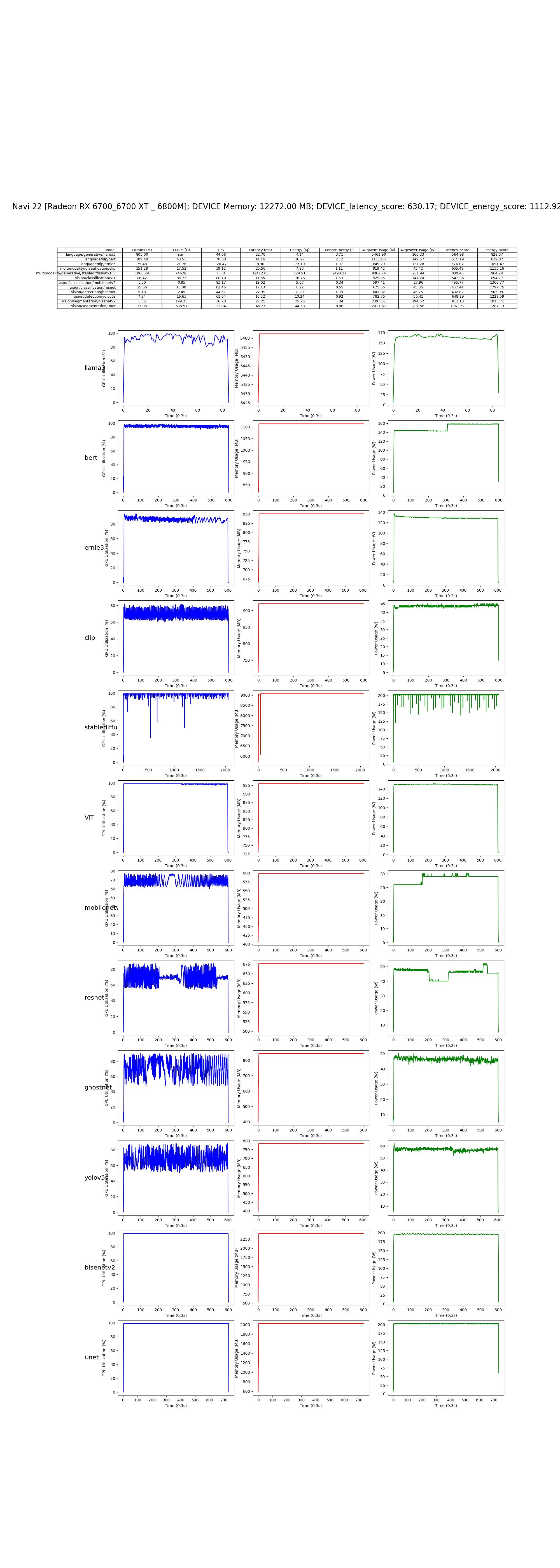
OpenCL (AMD)
OpenCL 在 AMD 平台与 NVIDIA 平台上的异同
核心相同点
-
开放标准:OpenCL 是一个跨平台的、开放的标准,支持不同厂商的硬件。无论是AMD还是NVIDIA,OpenCL都提供了统一的编程接口,开发者可以编写一次代码,然后在不同平台上运行,具备较强的可移植性。
-
异构计算模型:在两种平台上,OpenCL 都基于异构计算模型,利用 CPU 作为主机,GPU 作为加速器进行并行计算。开发者可以在这两种平台上实现多设备的协同计算。
-
编程模型:在AMD和NVIDIA平台上,OpenCL的内存模型和执行模型是统一的。无论在何种硬件上,开发者都可以定义内核函数,使用工作项(work-items)、工作组(work-groups)等概念来组织并行任务。
核心不同点
尽管OpenCL在两大平台上提供了一致的编程模型和接口,但在硬件优化、性能表现以及生态系统支持上存在显著差异。
1. 硬件优化差异
-
AMD 平台优化:AMD 对OpenCL有着长期的深度支持,并且在其GPU架构(如Radeon、Instinct系列)上做了较多的OpenCL优化,特别是在图形渲染、科学计算和深度学习推理等方面表现出色。由于AMD在异构计算领域的专注,它的硬件架构更适合使用OpenCL进行高效的并行计算。因此,在AMD的GPU上,OpenCL性能更为突出。
-
NVIDIA 平台优化:虽然NVIDIA也支持OpenCL,但它主要以CUDA作为其GPU并行计算的主要平台。由于NVIDIA的CUDA是专有技术,NVIDIA对CUDA进行了深入的硬件优化,而对OpenCL的优化力度相对较小。结果是在NVIDIA GPU上运行OpenCL程序时,通常性能不如CUDA程序。
2. 生态系统支持
-
AMD 的支持:AMD 在其Radeon和Instinct GPU系列上对OpenCL有着广泛的支持,并且随着ROCm(Radeon Open Compute)的引入,AMD在支持异构计算和并行任务中增强了OpenCL的功能。AMD的生态系统更多依赖于开源工具链,这使得开发者在使用OpenCL时拥有更大的灵活性和定制性。
-
NVIDIA 的支持:尽管NVIDIA支持OpenCL,但它的生态系统更多依赖于CUDA。CUDA具备丰富的库(如cuBLAS、cuDNN)和工具(如Nsight、CUDA Toolkit),为NVIDIA硬件上的AI和科学计算提供了强大的支持。因此,虽然NVIDIA提供OpenCL支持,但开发者在其硬件上通常更倾向于使用CUDA,因为CUDA具有更好的性能优化和开发支持。
3. 性能差异
-
在 AMD 平台上:由于AMD对OpenCL的深度优化以及其GPU架构设计的高并行性,OpenCL在AMD硬件上能够充分利用其计算资源。特别是在处理大规模并行计算任务(如图像处理、物理模拟、深度学习推理等)时,AMD的GPU在OpenCL上的表现往往优于NVIDIA的GPU。
-
在 NVIDIA 平台上:虽然OpenCL能在NVIDIA GPU上运行,但NVIDIA在设计和优化上主要面向CUDA。因此,即使在NVIDIA的高端GPU上,OpenCL程序的性能通常不及CUDA。此外,NVIDIA的硬件架构和OpenCL内存模型之间的匹配度相对较差,因此在一些复杂的并行任务中,性能差距可能更加明显。
4. 代码移植性
-
AMD 平台:由于AMD对OpenCL的优化和支持,开发者能够更轻松地在AMD平台上开发、优化和运行OpenCL程序,移植到其他平台时也能保持较好的性能表现。同时,AMD的ROCm平台也允许开发者将OpenCL与其他编程模型(如HIP)结合使用,以增强性能和兼容性。
-
NVIDIA 平台:虽然OpenCL在NVIDIA硬件上是跨平台的,但由于CUDA是NVIDIA的首选平台,许多开发者选择CUDA进行开发。这意味着在NVIDIA平台上开发OpenCL代码时,开发者通常无法利用NVIDIA硬件的全部潜力,并且在复杂应用中,性能优化的难度较高。
5. 开发工具支持
-
AMD 的开发工具:AMD 提供了丰富的开发工具来支持OpenCL的开发和优化。例如,AMD CodeXL(现为ROCm工具集的一部分)提供了强大的调试和性能分析功能,帮助开发者优化OpenCL应用在AMD GPU上的表现。
-
NVIDIA 的开发工具:尽管NVIDIA的开发工具主要针对CUDA优化,但它也为OpenCL提供了基本的开发支持。例如,NVIDIA Nsight能够分析和调试OpenCL代码,但这些工具通常在优化OpenCL程序时无法与CUDA开发时的工具那样深入和高效。
技术栈架构
1. 系统软件层
- 设备驱动程序:
- 为特定硬件(如 GPU、CPU、FPGA)提供底层支持
- 实现 OpenCL 规范定义的功能
- 处理设备特定的优化和功能
- OpenCL ICD (Installable Client Driver):
- 提供对多个 OpenCL 实现的支持
- 允许在同一系统上共存多个 OpenCL 供应商的实现
- 管理不同 OpenCL 实现之间的切换和交互
2. 运行时环境层
- OpenCL Runtime:
- 提供 OpenCL API 的实现
- 管理设备、上下文、命令队列和内存对象
- 处理内核编译和执行
- 协调主机和设备之间的数据传输
- 支持事件和同步机制
3. 编程模型和语言层
- OpenCL C/C++:
- 基于 C99 标准的编程语言,用于编写 OpenCL 内核
- 支持向量数据类型和内置函数
- 提供内存模型和同步原语
- 允许编写可在各种设备上执行的并行代码
- OpenCL C++ 包装器:
- 为 C++ 程序员提供面向对象的 API
- 简化内存管理和错误处理
- 提供更现代的 C++ 接口
4. 计算库层
- clBLAS:
- OpenCL 实现的基本线性代数子程序(BLAS)库
- 提供矩阵和向量操作的高性能实现
- 支持多种设备类型
- clDNN (Compute Library for Deep Neural Networks):
- 用于深度学习的 OpenCL 加速库
- 提供常见的神经网络层和操作
- 优化for各种硬件平台
5. 框架模型层
- TensorFlow with OpenCL:
- 通过 ComputeCpp 或其他 OpenCL 后端支持 OpenCL
- 允许在支持 OpenCL 的设备上运行 TensorFlow 模型
- Caffe with OpenCL:
- 使用 OpenCL 后端的 Caffe 深度学习框架
- 支持在各种 OpenCL 设备上训练和推理
- OpenCV with OpenCL:
- 计算机视觉库,集成了 OpenCL 支持
- 利用 OpenCL 加速图像和视频处理操作
- ArrayFire:
- 高性能计算库,支持 OpenCL 后端
- 提供线性代数、信号处理和计算机视觉功能
- 简化了 OpenCL 编程,提供高级抽象

关系解析
OpenCL作为一个开放的异构计算框架,在模型层面支持硬件加速、跨设备兼容性和性能优化。它的核心组件包括OpenCL ICD、OpenCL Runtime和OpenCL C/C++语言。
OpenCL ICD (Installable Client Driver) 是一个关键组件,它允许多个OpenCL实现共存,提供了一个统一的接口来管理不同厂商的OpenCL实现。这种设计极大地增强了OpenCL的灵活性和可扩展性,使得开发者可以在不同的硬件平台上无缝切换。OpenCL Runtime负责管理设备、内存和任务调度等核心功能。它处理内存分配、数据传输、内核编译和执行等底层操作,为开发者提供了一个抽象层,简化了异构计算的复杂性。Runtime与ICD紧密协作,确保了OpenCL应用程序的高效运行。
在编程语言方面,OpenCL C/C++扩展了标准C/C++,增加了并行计算所需的特性。它支持向量数据类型、内存模型和并行编程构造,使得开发者能够充分利用异构计算资源。OpenCL 2.1引入了SPIR-V中间表示,进一步增强了跨平台兼容性和编译优化。clBLAS和clDNN是基于OpenCL的重要库,分别针对基础线性代数子程序和深度神经网络计算进行了优化。这些库充分利用了OpenCL的并行计算能力,为科学计算和机器学习应用提供了高性能解决方案。OpenCL与其他技术的集成也是其强大之处。例如,深度学习框架如PyTorch可以利用OpenCL进行GPU加速,而OpenCL本身也支持与CUDA等其他并行计算框架的互操作。
总的来说,OpenCL通过其灵活的架构、强大的运行时系统和丰富的编程接口,为异构计算提供了一个全面的解决方案。它不仅支持跨平台开发,还能够充分发挥各种计算设备的性能潜力,在高性能计算、图像处理、科学模拟等领域发挥着重要作用。OpenCL的生态系统持续发展,不断适应新的硬件架构和计算需求,为未来的并行计算和异构系统开发铺平了道路。
系统软件层
下面是一个使用 OpenCL API 列出系统中所有可用的 AMD 设备的示例代码。该代码将获取设备名称、驱动版本、计算单元数量和全局内存大小,并创建和销毁 OpenCL 上下文。
示例代码:
#include <iostream>
#include <CL/cl.h>

// Check the return value of OpenCL functions and print error message on failure
void checkOpenCLErrors(cl_int result) {
    if (result != CL_SUCCESS) {
        std::cerr << "OpenCL Error: " << result << std::endl;
        exit(EXIT_FAILURE);
    }
}

// Print information about an OpenCL device
void printDeviceInfo(cl_device_id device) {
    char deviceName[256];
    checkOpenCLErrors(clGetDeviceInfo(device, CL_DEVICE_NAME, sizeof(deviceName), deviceName, nullptr));

    cl_uint computeUnits;
    checkOpenCLErrors(clGetDeviceInfo(device, CL_DEVICE_MAX_COMPUTE_UNITS, sizeof(computeUnits), &computeUnits, nullptr));

    cl_uint driverVersionSize;
    checkOpenCLErrors(clGetDeviceInfo(device, CL_DRIVER_VERSION, 0, nullptr, &driverVersionSize));
    std::string driverVersion(driverVersionSize, '\0');
    checkOpenCLErrors(clGetDeviceInfo(device, CL_DRIVER_VERSION, driverVersionSize, &driverVersion[0], nullptr));

    cl_ulong globalMemorySize;
    checkOpenCLErrors(clGetDeviceInfo(device, CL_DEVICE_GLOBAL_MEM_SIZE, sizeof(globalMemorySize), &globalMemorySize, nullptr));

    // Print device details
    std::cout << "Device Name: " << deviceName << std::endl;
    std::cout << "Max Compute Units: " << computeUnits << std::endl;
    std::cout << "Driver Version: " << driverVersion << std::endl;
    std::cout << "Total Global Memory: " << globalMemorySize / (1024 * 1024) << " MB" << std::endl;
}

int main() {
    cl_int result;

    // Get the number of available OpenCL platforms
    cl_uint platformCount;
    result = clGetPlatformIDs(0, nullptr, &platformCount);
    checkOpenCLErrors(result);

    std::vector<cl_platform_id> platforms(platformCount);
    result = clGetPlatformIDs(platformCount, platforms.data(), nullptr);
    checkOpenCLErrors(result);

    cl_platform_id amdPlatform = nullptr;

    // Check for AMD platform
    for (cl_platform_id platform : platforms) {
        char platformName[256];
        checkOpenCLErrors(clGetPlatformInfo(platform, CL_PLATFORM_NAME, sizeof(platformName), platformName, nullptr));
        if (std::string(platformName).find("AMD") != std::string::npos) {
            amdPlatform = platform;
            break;
        }
    }

    if (amdPlatform == nullptr) {
        std::cerr << "No AMD platform found." << std::endl;
        return -1;
    }

    // Get the number of devices for the AMD platform
    cl_uint deviceCount;
    checkOpenCLErrors(clGetDeviceIDs(amdPlatform, CL_DEVICE_TYPE_GPU, 0, nullptr, &deviceCount));
    std::cout << "Number of AMD GPU Devices: " << deviceCount << std::endl;

    std::vector<cl_device_id> devices(deviceCount);
    checkOpenCLErrors(clGetDeviceIDs(amdPlatform, CL_DEVICE_TYPE_GPU, deviceCount, devices.data(), nullptr));

    // Iterate through each device and print its information
    for (cl_device_id device : devices) {
        printDeviceInfo(device);
        std::cout << std::endl;
    }

    // Create an OpenCL context
    cl_context context = clCreateContext(nullptr, deviceCount, devices.data(), nullptr, nullptr, &result);
    checkOpenCLErrors(result);
    std::cout << "OpenCL context created successfully." << std::endl;

    // Cleanup
    checkOpenCLErrors(clReleaseContext(context));

    return 0;
}
结果:
Number of AMD GPU Devices: 1
Device Name: AMD Radeon RX 7900 XTX
运行时环境层
在现代计算架构中,OpenCL Runtime 作为一个核心软件组件,承担着在不同平台和硬件设备上执行 OpenCL 程序的责任。它不仅为开发者提供了一系列 API 和工具,帮助管理计算设备,还支持创建、编译和调度 OpenCL 程序,进行内存管理。本文将深入探讨 OpenCL Runtime 的各个功能模块,包括设备管理、上下文创建、内存管理、程序编译与执行、命令队列管理以及事件和同步机制。
在接下来的内容中,我们将通过一个示例程序来演示如何在 AMD 平台上使用 OpenCL Runtime 实现一个简单的向量加法操作。
代码示例如下:
#define CL_TARGET_OPENCL_VERSION 220
#include <CL/cl.h>
#include <stdio.h>
#include <stdlib.h>
#include <cstring>

#define ARRAY_SIZE 1024

// OpenCL kernel code for vector addition
const char* kernelSource = "__kernel void vec_add(__global float* A, __global float* B, __global float* C) { \
                                int id = get_global_id(0); \
                                C[id] = A[id] + B[id]; \
                            }";

int main() {
    cl_platform_id platform_id = NULL;
    cl_device_id device_id;
    cl_context context;
    cl_command_queue queue;
    cl_program program;
    cl_kernel kernel;
    cl_int ret;

    // Arrays on the host
    float A[ARRAY_SIZE], B[ARRAY_SIZE], C[ARRAY_SIZE];
    for (int i = 0; i < ARRAY_SIZE; i++) {
        A[i] = i;
        B[i] = i * 2;
    }

    // 1. Get the number of platforms
    cl_uint num_platforms;
    ret = clGetPlatformIDs(0, NULL, &num_platforms);
    if (ret != CL_SUCCESS) {
        printf("Failed to get platform IDs\n");
        return -1;
    }

    cl_platform_id* platforms = (cl_platform_id*)malloc(num_platforms * sizeof(cl_platform_id));
    ret = clGetPlatformIDs(num_platforms, platforms, NULL);
    if (ret != CL_SUCCESS) {
        printf("Failed to get platforms\n");
        free(platforms);
        return -1;
    }

    // Try to find the AMD platform
    for (cl_uint i = 0; i < num_platforms; i++) {
        char platform_name[128];
        clGetPlatformInfo(platforms[i], CL_PLATFORM_NAME, sizeof(platform_name), platform_name, NULL);
        printf("Platform %d: %s\n", i, platform_name);

        if (strstr(platform_name, "AMD") != NULL) {
            platform_id = platforms[i];
            printf("Selected AMD platform: %s\n", platform_name);
            break;
        }
    }

    if (!platform_id) {
        printf("AMD platform not found\n");
        free(platforms);
        return -1;
    }

    // 2. Get the GPU device from the selected AMD platform
    ret = clGetDeviceIDs(platform_id, CL_DEVICE_TYPE_GPU, 1, &device_id, NULL);
    if (ret != CL_SUCCESS) {
        printf("Failed to get GPU device ID from AMD platform, error code: %d\n", ret);
        free(platforms);
        return -1;
    }

    // Print the selected device
    char device_name[128];
    clGetDeviceInfo(device_id, CL_DEVICE_NAME, sizeof(device_name), device_name, NULL);
    printf("Selected device: %s\n", device_name);

    // 3. Create a context
    context = clCreateContext(NULL, 1, &device_id, NULL, NULL, &ret);
    if (ret != CL_SUCCESS) {
        printf("Failed to create context\n");
        free(platforms);
        return -1;
    }
    printf("Context created successfully.\n");

    // 4. Create a command queue
    queue = clCreateCommandQueueWithProperties(context, device_id, 0, &ret);
    if (ret != CL_SUCCESS) {
        printf("Failed to create command queue\n");
        free(platforms);
        return -1;
    }
    printf("Command queue created successfully.\n");

    // 5. Create a program from the kernel source
    program = clCreateProgramWithSource(context, 1, &kernelSource, NULL, &ret);
    if (ret != CL_SUCCESS) {
        printf("Failed to create program\n");
        free(platforms);
        return -1;
    }
    printf("Program created successfully.\n");

    // 6. Build the program
    ret = clBuildProgram(program, 1, &device_id, NULL, NULL, NULL);
    if (ret != CL_SUCCESS) {
        printf("Failed to build program\n");
        char log[1024];
        clGetProgramBuildInfo(program, device_id, CL_PROGRAM_BUILD_LOG, sizeof(log), log, NULL);
        printf("Build log:\n%s\n", log);
        free(platforms);
        return -1;
    }
    printf("Program built successfully.\n");

    // 7. Create the kernel
    kernel = clCreateKernel(program, "vec_add", &ret);
    if (ret != CL_SUCCESS) {
        printf("Failed to create kernel\n");
        free(platforms);
        return -1;
    }
    printf("Kernel created successfully.\n");

    // 8. Create buffers for the input and output arrays
    cl_mem buffer_A = clCreateBuffer(context, CL_MEM_READ_ONLY, ARRAY_SIZE * sizeof(float), NULL, &ret);
    cl_mem buffer_B = clCreateBuffer(context, CL_MEM_READ_ONLY, ARRAY_SIZE * sizeof(float), NULL, &ret);
    cl_mem buffer_C = clCreateBuffer(context, CL_MEM_WRITE_ONLY, ARRAY_SIZE * sizeof(float), NULL, &ret);

    if (ret != CL_SUCCESS) {
        printf("Failed to create buffers\n");
        free(platforms);
        return -1;
    }
    printf("Buffers created successfully.\n");

    // 9. Copy the input data to the respective memory buffers
    ret = clEnqueueWriteBuffer(queue, buffer_A, CL_TRUE, 0, ARRAY_SIZE * sizeof(float), A, 0, NULL, NULL);
    ret |= clEnqueueWriteBuffer(queue, buffer_B, CL_TRUE, 0, ARRAY_SIZE * sizeof(float), B, 0, NULL, NULL);
    if (ret != CL_SUCCESS) {
        printf("Failed to write to buffers\n");
        free(platforms);
        return -1;
    }
    printf("Data written to buffers successfully.\n");

    // 10. Set the kernel arguments
    ret = clSetKernelArg(kernel, 0, sizeof(cl_mem), (void*)&buffer_A);
    ret |= clSetKernelArg(kernel, 1, sizeof(cl_mem), (void*)&buffer_B);
    ret |= clSetKernelArg(kernel, 2, sizeof(cl_mem), (void*)&buffer_C);
    if (ret != CL_SUCCESS) {
        printf("Failed to set kernel arguments\n");
        free(platforms);
        return -1;
    }
    printf("Kernel arguments set successfully.\n");

    // 11. Execute the kernel
    size_t global_size = ARRAY_SIZE;
    ret = clEnqueueNDRangeKernel(queue, kernel, 1, NULL, &global_size, NULL, 0, NULL, NULL);
    if (ret != CL_SUCCESS) {
        printf("Failed to enqueue kernel\n");
        free(platforms);
        return -1;
    }
    printf("Kernel enqueued successfully.\n");

    // 12. Read the output buffer back to the host
    ret = clEnqueueReadBuffer(queue, buffer_C, CL_TRUE, 0, ARRAY_SIZE * sizeof(float), C, 0, NULL, NULL);
    if (ret != CL_SUCCESS) {
        printf("Failed to read from buffer\n");
        free(platforms);
        return -1;
    }
    printf("Data read from buffer successfully.\n");

    // Output the results
    printf("Result:\n");
    for (int i = 0; i < 10; i++) {
        printf("C[%d] = %f\n", i, C[i]);
    }

    // 13. Clean up
    clReleaseMemObject(buffer_A);
    clReleaseMemObject(buffer_B);
    clReleaseMemObject(buffer_C);
    clReleaseKernel(kernel);
    clReleaseProgram(program);
    clReleaseCommandQueue(queue);
    clReleaseContext(context);
    free(platforms);

    printf("Resources released successfully.\n");
    return 0;
}
结果:
Platform 0: Intel(R) OpenCL
Platform 1: AMD Accelerated Parallel Processing
Selected AMD platform: AMD Accelerated Parallel Processing
Selected device: AMD Radeon RX 7900 XTX
Context created successfully.
Command queue created successfully.
Program created successfully.
Program built successfully.
Kernel created successfully.
Buffers created successfully.
Data written to buffers successfully.
Kernel arguments set successfully.
Kernel enqueued successfully.
Data read from buffer successfully.
Result:
C[0] = 0.000000
C[1] = 3.000000
C[2] = 6.000000
C[3] = 9.000000
C[4] = 12.000000
C[5] = 15.000000
C[6] = 18.000000
C[7] = 21.000000
C[8] = 24.000000
编程模型和语言层
OpenCL 是由 Khronos Group 管理的跨平台并行编程框架,它在包括 CPU、GPU 和 FPGA 等多种设备上提供了统一的编程接口。对于 AMD 平台,OpenCL 支持充分利用 AMD GPU 的计算能力,允许开发者在 AMD 硬件上高效执行并行计算任务。
1. OpenCL 的核心编程特性
与 CUDA 类似,OpenCL 强调对设备内存和计算资源的精确控制。AMD 平台上的 OpenCL 编程模型具有以下关键特性:
- 平台模型 :OpenCL 的平台模型由主机(Host)和一个或多个设备(Device)组成。在 AMD 平台上,主机通常是 CPU,设备是 AMD GPU。开发者需要显式管理主机与设备之间的交互。
- 上下文和命令队列 :在 AMD 平台上,OpenCL 的上下文(Context)管理设备、内核程序和内存对象的生命周期。命令队列(Command Queue)则用于调度内核执行和数据传输操作。在 AMD GPU 上,命令队列可以并行化执行任务,支持多任务并发处理。
- 内核(Kernel)函数 :在 OpenCL 中,计算核心是内核函数,它定义了在设备上并行执行的代码。内核函数使用
__kernel修饰符表明其将在设备上执行,结构与其他平台相同。
__kernel void vectorAdd(__global const float* A, __global const float* B, __global float* C, int N) {
    int i = get_global_id(0);
    if (i < N) C[i] = A[i] + B[i];
}
这个简单的内核展示了如何通过 OpenCL 执行并行向量加法运算,get_global_id(0) 获取当前工作项的唯一 ID,用于计算索引。
- 内存模型 :OpenCL 内存模型包含全局内存、常量内存、局部内存和私有内存。工作项可以访问这些内存区域,但不同内存区域的性能特性不同。例如,局部内存具有较快的访问速度,因此在 AMD GPU 上优化内存访问时,合理使用局部内存可以显著提高性能。
- 设备和内存管理 :与 CUDA 类似,OpenCL 需要手动管理主机和设备之间的数据传输。通过
clCreateBuffer创建缓冲区对象,使用clEnqueueWriteBuffer和clEnqueueReadBuffer在主机和设备之间传输数据。
2. 算子编写示例:矩阵乘法
矩阵乘法是并行计算中的经典操作之一,以下是一个在 OpenCL 中的并行矩阵乘法内核:
__kernel void matrixMul(__global float* A, __global float* B, __global float* C, int N) {
    int row = get_global_id(1);
    int col = get_global_id(0);
    float result = 0.0;
    if (row < N && col < N) {
        for (int i = 0; i < N; ++i) {
            result += A[row * N + i] * B[i * N + col];
        }
        C[row * N + col] = result;
    }
}
在 AMD GPU 上,get_global_id(0) 和 get_global_id(1) 用于获取工作项的横纵坐标,每个工作项负责计算结果矩阵中的一个元素。由于 AMD GPU 通常具有大量并行计算单元,这种并行计算能够充分发挥硬件的计算性能。
3. 并行计算模型介绍
OpenCL 的并行计算模型包括工作项(Work-Item)和工作组(Work-Group)。多个工作项组成工作组,每个工作项独立执行一小部分计算。工作组之间是独立的,但同一工作组内的工作项可以共享局部内存并进行同步操作。
- 全局与局部内存 :AMD GPU 提供高带宽的全局内存访问和更快的局部内存访问。合理利用局部内存可以极大地减少全局内存访问的延迟,从而提升性能。局部内存的高效使用尤其在矩阵乘法等算法中至关重要。
- 命令队列与同步 :在 OpenCL 中,主机通过命令队列提交计算任务。通过事件机制,开发者可以在任务完成后触发事件,控制任务的调度和设备资源的使用。在 AMD GPU 上,这种机制可以帮助协调多任务的并行执行,提高设备利用率。
4. OpenCL 与 CUDA 的对比
在 AMD 平台上,OpenCL 提供了一个灵活的异构计算模型,但与 CUDA 相比,仍然有一些区别:
- 跨平台性 :OpenCL 是跨平台标准,能够在 AMD、Intel、NVIDIA 等多种硬件上运行。而 CUDA 是 NVIDIA 专有的技术,仅限于 NVIDIA 硬件。对于需要在 AMD GPU 上执行异构计算的应用,OpenCL 是不可或缺的。
- 性能优化 :尽管 OpenCL 提供跨平台支持,AMD 对 OpenCL 的优化与 NVIDIA 对 CUDA 的优化存在差异。AMD 对其硬件架构的深入理解使其能够通过 OpenCL 实现高效的计算,特别是在深度学习和 AI 领域,AMD 的 MI250、MI300 等 GPU 提供了优秀的性能。
- 编程复杂度 :与 CUDA 相比,OpenCL 代码编写相对复杂。开发者需要手动管理设备上下文、内存分配和内核调度。然而,AMD 提供了开发工具和优化库,帮助开发者更好地使用 OpenCL 在其硬件上实现高效的并行计算。
5. OpenCL 在 AI 开发中的应用
OpenCL 在 AI 和深度学习中的应用主要体现在跨平台计算和嵌入式计算设备中:
- 跨平台通用性 :对于需要在不同硬件平台上运行的 AI 应用,OpenCL 提供了统一的并行计算支持。比如在需要同时支持 CPU、AMD GPU 的场景下,OpenCL 能够保证程序的兼容性。
- AI 和深度学习库优化 :AMD 通过 ROCm 软件栈对 OpenCL 进行了大量优化,使其能够在深度学习和 AI 应用中表现出色。ROCm 提供了诸如 MIOpen 等加速库,使得 OpenCL 在 AI 推理和训练任务中能够高效执行。
6. 总结
通过理解 AMD OpenCL 的编程模型和并行计算特性,开发者可以在 AMD 硬件平台上构建高效的异构计算应用,充分利用 AMD GPU 的强大计算能力。
计算库层
clBLAS 是一个开源的高性能线性代数库,专为 OpenCL 平台设计,支持多种基本线性代数操作,如矩阵乘法和矩阵-向量乘法。clBLAS 利用 OpenCL 的并行计算能力,提供灵活的内存管理和高效的内核优化,显著提升线性代数运算的性能。
参考仓库地址:clBLAS
clblasChemm 展示了如何使用 clBLAS 进行复数矩阵的乘法操作。
示例代码如下:
/* ************************************************************************
 * Copyright 2013 Advanced Micro Devices, Inc.
 *
 * Licensed under the Apache License, Version 2.0 (the "License");
 * you may not use this file except in compliance with the License.
 * You may obtain a copy of the License at
 *
 * http://www.apache.org/licenses/LICENSE-2.0
 *
 * Unless required by applicable law or agreed to in writing, software
 * distributed under the License is distributed on an "AS IS" BASIS,
 * WITHOUT WARRANTIES OR CONDITIONS OF ANY KIND, either express or implied.
 * See the License for the specific language governing permissions and
 * limitations under the License.
 * ************************************************************************/


#include <sys/types.h>
#include <stdio.h>
#include <string.h>

/* Include CLBLAS header. It automatically includes needed OpenCL header,
 * so we can drop out explicit inclusion of cl.h header.
 */
#include <clBLAS.h>

/* This example uses predefined matrices and their characteristics for
 * simplicity purpose.
 */
static const clblasOrder order = clblasRowMajor;

#define M  4
#define N  3

static const cl_float2 alpha = {{10, 10}};

static const clblasSide side = clblasLeft;
static const clblasUplo uplo = clblasLower;
static const cl_float2 A[M*M] = {
    {{11, 12}}, {{-1, -1}}, {{-1, -1}}, {{-1, -1}},
    {{21, 22}}, {{22, 23}}, {{-1, -1}}, {{-1, -1}},
    {{31, 32}}, {{32, 33}}, {{33, 34}}, {{-1, -1}},
    {{41, 61}}, {{42, 62}}, {{43, 73}}, {{44, 23}}
};
static const size_t lda = M;

static const cl_float2 B[M*N] = {
    {{11, -21}},  {{-12, 23}}, {{13, 33}},
    {{21, 12}},   {{22, -10}}, {{23, 5}},
    {{31, 1}},    {{-32, 65}}, {{33, -1}},
    {{1, 41}},    {{-33, 42}}, {{12, 43}},
};
static const size_t ldb = N;

static const cl_float2 beta = {{20, 20}};

static cl_float2 C[M*N] = {
    {{11, 11}},  {{-12, 12}}, {{13, 33}},
    {{21, -32}}, {{22,  -1}}, {{23, 0}},
    {{31, 13}},  {{-32, 78}}, {{33, 45}},
    {{41, 14}},  {{0,   42}}, {{43, -1}},
};
static const size_t ldc = N;

static void
printResult(void)
{
    size_t i, j, nrows;

    printf("Result:\n");

    nrows = (sizeof(C) / sizeof(cl_float2)) / ldc;
    for (i = 0; i < nrows; i++) {
        for (j = 0; j < ldc; j++) {
            printf("<%9.2f, %-9.2f> ", CREAL(C[i * ldc + j]), CIMAG(C[i*ldc + j]));
        }
        printf("\n");
    }
}

int
main(void)
{
    cl_int err;
    cl_platform_id platform = 0;
    cl_device_id device = 0;
    cl_context_properties props[3] = { CL_CONTEXT_PLATFORM, 0, 0 };
    cl_context ctx = 0;
    cl_command_queue queue = 0;
    cl_mem bufA, bufB, bufC;
    cl_event event = NULL;
    int ret = 0;

    /* Setup OpenCL environment. */
    err = clGetPlatformIDs(1, &platform, NULL);
    if (err != CL_SUCCESS) {
        printf( "clGetPlatformIDs() failed with %d\n", err );
        return 1;
    }

    err = clGetDeviceIDs(platform, CL_DEVICE_TYPE_GPU, 1, &device, NULL);
    if (err != CL_SUCCESS) {
        printf( "clGetDeviceIDs() failed with %d\n", err );
        return 1;
    }

    props[1] = (cl_context_properties)platform;
    ctx = clCreateContext(props, 1, &device, NULL, NULL, &err);
    if (err != CL_SUCCESS) {
        printf( "clCreateContext() failed with %d\n", err );
        return 1;
    }

    queue = clCreateCommandQueue(ctx, device, 0, &err);
    if (err != CL_SUCCESS) {
        printf( "clCreateCommandQueue() failed with %d\n", err );
        clReleaseContext(ctx);
        return 1;
    }

    /* Setup clblas. */
    err = clblasSetup();
    if (err != CL_SUCCESS) {
        printf("clblasSetup() failed with %d\n", err);
        clReleaseCommandQueue(queue);
        clReleaseContext(ctx);
        return 1;
    }

    /* Prepare OpenCL memory objects and place matrices inside them. */
    bufA = clCreateBuffer(ctx, CL_MEM_READ_ONLY, M * M * sizeof(*A),
                          NULL, &err);
    bufB = clCreateBuffer(ctx, CL_MEM_READ_ONLY, M * N * sizeof(*B),
                          NULL, &err);
    bufC = clCreateBuffer(ctx, CL_MEM_READ_WRITE, M * N * sizeof(*C),
                          NULL, &err);

    err = clEnqueueWriteBuffer(queue, bufA, CL_TRUE, 0,
        M * M * sizeof(*A), A, 0, NULL, NULL);
    err = clEnqueueWriteBuffer(queue, bufB, CL_TRUE, 0,
        M * N * sizeof(*B), B, 0, NULL, NULL);
    err = clEnqueueWriteBuffer(queue, bufC, CL_TRUE, 0,
        M * N * sizeof(*C), C, 0, NULL, NULL);

    /* Call clblas function. */
    err = clblasChemm(order, side, uplo, M, N, alpha, bufA,
                         0, lda, bufB, 0, ldb, beta, bufC, 0, ldc, 1, &queue,
                         0, NULL, &event);
    if (err != CL_SUCCESS) {
        printf("clblasSsymm() failed with %d\n", err);
        ret = 1;
    }
    else {
        /* Wait for calculations to be finished. */
        err = clWaitForEvents(1, &event);

        /* Fetch results of calculations from GPU memory. */
        err = clEnqueueReadBuffer(queue, bufC, CL_TRUE, 0, M * N * sizeof(*C),
                                  C, 0, NULL, NULL);

        /* At this point you will get the result of SYMM placed in C array. */
        printResult();
    }

    /* Release OpenCL events. */
    clReleaseEvent(event);

    /* Release OpenCL memory objects. */
    clReleaseMemObject(bufC);
    clReleaseMemObject(bufB);
    clReleaseMemObject(bufA);

    /* Finalize work with clblas. */
    clblasTeardown();

    /* Release OpenCL working objects. */
    clReleaseCommandQueue(queue);
    clReleaseContext(ctx);

    return ret;
}
结果:
Result:
< 41430.00, 46230.00 > <-39740.00, 87400.00 > < 48960.00, 48400.00 >
< 41360.00, 54760.00 > <-48340.00, 90520.00 > < 32620.00, 53220.00 >
< 28830.00, 79370.00 > <-67980.00, 77040.00 > < 13400.00, 81160.00 >
<-24980.00, 90100.00 > <-114700.00, -43780.00> <-67560.00, 93200.00 >
clblasScopy 是 clBLAS 库中的一个函数,它是 BLAS 标准中 scopy 函数的 OpenCL 版本。scopy 函数的作用是复制浮点数组。在 clBLAS 中,clblasScopy 用于将一个浮点数组复制到另一个浮点数组,这两个数组可以位于不同的内存区域。
示例代码如下:
/* ************************************************************************
 * Copyright 2013 Advanced Micro Devices, Inc.
 *
 * Licensed under the Apache License, Version 2.0 (the "License");
 * you may not use this file except in compliance with the License.
 * You may obtain a copy of the License at
 *
 * http://www.apache.org/licenses/LICENSE-2.0
 *
 * Unless required by applicable law or agreed to in writing, software
 * distributed under the License is distributed on an "AS IS" BASIS,
 * WITHOUT WARRANTIES OR CONDITIONS OF ANY KIND, either express or implied.
 * See the License for the specific language governing permissions and
 * limitations under the License.
 * ************************************************************************/

#include <sys/types.h>
#include <stdio.h>
#include <string.h>
#include <math.h>

/* Include CLBLAS header. It automatically includes needed OpenCL header,
 * so we can drop out explicit inclusion of cl.h header.
 */
#include <clBLAS.h>

/* This example uses predefined matrices and their characteristics for
 * simplicity purpose.
 */
static const size_t N = 7;
static cl_float X[] = {
    11,
    21,
    31,
    41,
    51,
    61,
    71,
};
static const int incx = 1;

static cl_float Y[] = {
    0,
    2,
    0,
    0,
    0,
    5,
    0,
};
static const int incy = 1;


static void
printResult(void)
{
    size_t i;
    printf("\nResult:\n");

    printf(" X\n");
    for (i = 0; i < N; i++) {
            printf("\t%f\n", X[i]);
    }

    printf("Y\n");
    for (i = 0; i < N; i++) {
            printf("\t%f\n", Y[i]);
    }
}

int
main(void)
{
    cl_int err;
    cl_platform_id platform = 0;
    cl_device_id device = 0;
    cl_context_properties props[3] = { CL_CONTEXT_PLATFORM, 0, 0 };
    cl_context ctx = 0;
    cl_command_queue queue = 0;
    cl_mem bufX, bufY;
    cl_event event = NULL;
    int ret = 0;
    int lenX = 1 + (N-1)*abs(incx);
    int lenY = 1 + (N-1)*abs(incy);

    /* Setup OpenCL environment. */
    err = clGetPlatformIDs(1, &platform, NULL);
    if (err != CL_SUCCESS) {
        printf( "clGetPlatformIDs() failed with %d\n", err );
        return 1;
    }

    err = clGetDeviceIDs(platform, CL_DEVICE_TYPE_GPU, 1, &device, NULL);
    if (err != CL_SUCCESS) {
        printf( "clGetDeviceIDs() failed with %d\n", err );
        return 1;
    }

    props[1] = (cl_context_properties)platform;
    ctx = clCreateContext(props, 1, &device, NULL, NULL, &err);
    if (err != CL_SUCCESS) {
        printf( "clCreateContext() failed with %d\n", err );
        return 1;
    }

    queue = clCreateCommandQueue(ctx, device, 0, &err);
    if (err != CL_SUCCESS) {
        printf( "clCreateCommandQueue() failed with %d\n", err );
        clReleaseContext(ctx);
        return 1;
    }

    /* Setup clblas. */
    err = clblasSetup();
    if (err != CL_SUCCESS) {
        printf("clblasSetup() failed with %d\n", err);
        clReleaseCommandQueue(queue);
        clReleaseContext(ctx);
        return 1;
    }

    /* Prepare OpenCL memory objects and place matrices inside them. */
    bufX = clCreateBuffer(ctx, CL_MEM_READ_ONLY, (lenX*sizeof(cl_float)), NULL, &err);
    bufY = clCreateBuffer(ctx, CL_MEM_READ_WRITE, (lenY*sizeof(cl_float)), NULL, &err);

    err = clEnqueueWriteBuffer(queue, bufX, CL_TRUE, 0, (lenX*sizeof(cl_float)), X, 0, NULL, NULL);
    err = clEnqueueWriteBuffer(queue, bufY, CL_TRUE, 0, (lenY*sizeof(cl_float)), Y, 0, NULL, NULL);

    /* Call clblas function. */
    err = clblasScopy( N, bufX, 0, incx, bufY, 0, incy, 1, &queue, 0, NULL, &event);
    if (err != CL_SUCCESS) {
        printf("clblasScopy() failed with %d\n", err);
        ret = 1;
    }
    else {
        /* Wait for calculations to be finished. */
        err = clWaitForEvents(1, &event);

        /* Fetch results of calculations from GPU memory. */
        err = clEnqueueReadBuffer(queue, bufX, CL_TRUE, 0, (lenX*sizeof(cl_float)),
                                    X, 0, NULL, NULL);
        err = clEnqueueReadBuffer(queue, bufY, CL_TRUE, 0, (lenY*sizeof(cl_float)),
                                    Y, 0, NULL, NULL);

        /* At this point you will get the result of SSWAP placed in vector Y. */
        printResult();
    }

    /* Release OpenCL events. */
    clReleaseEvent(event);

    /* Release OpenCL memory objects. */
    clReleaseMemObject(bufY);
    clReleaseMemObject(bufX);

    /* Finalize work with clblas. */
    clblasTeardown();

    /* Release OpenCL working objects. */
    clReleaseCommandQueue(queue);
    clReleaseContext(ctx);

    return ret;
}
结果:
Result:
 X
        11.000000
        21.000000
        31.000000
        41.000000
        51.000000
        61.000000
        71.000000
Y
        11.000000
        21.000000
        31.000000
        41.000000
        51.000000
        61.000000
        71.000000
clblasSgemm 是 clBLAS 库中的一个函数,用于执行单精度浮点数的矩阵乘法。Sgemm 代表单精度(Single precision)和矩阵乘法(GEneral Matrix-Matrix multiplication)。这个函数是 BLAS 库中最基本的函数之一,广泛用于科学计算、工程模拟、数据分析和机器学习等领域。
示例代码如下:
#include <stdio.h>
#include <stdlib.h>
#include <CL/cl.h>
#include <clBLAS.h>
#include <sys/time.h>

#define M 320
#define N 320
#define K 320
#define ITERATIONS 300

static const clblasOrder order = clblasRowMajor;
static const cl_float alpha = 1.0f;
static const clblasTranspose transA = clblasNoTrans;
static const clblasTranspose transB = clblasNoTrans;
static const cl_float beta = 0.0f;

static cl_float A[M*K];
static cl_float B[K*N];
static cl_float C[M*N];
static cl_float result[M*N];

void initMatrix(cl_float *mat, size_t size, cl_float value) {
    for (size_t i = 0; i < size; i++) {
        mat[i] = value;
    }
}

double getCurrentTimeInMilliseconds() {
    struct timeval time;
    gettimeofday(&time, NULL);
    return time.tv_sec * 1000.0 + time.tv_usec / 1000.0;
}

int main(void) {
    cl_int err;
    cl_platform_id platform = 0;
    cl_device_id device = 0;
    cl_context_properties props[3] = { CL_CONTEXT_PLATFORM, 0, 0 };
    cl_context ctx = 0;
    cl_command_queue queue = 0;
    cl_mem bufA, bufB, bufC;
    cl_event event = NULL;

    printf("[Matrix Multiply Using clBLAS] - Starting...\n");

    // Initialize matrices
    initMatrix(A, M * K, 1.0f);
    initMatrix(B, K * N, 0.01f);
    initMatrix(C, M * N, 0.0f);

    // Setup OpenCL environment
    err = clGetPlatformIDs(1, &platform, NULL);
    err = clGetDeviceIDs(platform, CL_DEVICE_TYPE_GPU, 1, &device, NULL);

    // Create OpenCL context and command queue
    props[1] = (cl_context_properties)platform;
    ctx = clCreateContext(props, 1, &device, NULL, NULL, &err);
    queue = clCreateCommandQueue(ctx, device, 0, &err);

    // Setup clBLAS
    clblasSetup();

    // Prepare OpenCL memory objects
    bufA = clCreateBuffer(ctx, CL_MEM_READ_ONLY, M * K * sizeof(*A), NULL, &err);
    bufB = clCreateBuffer(ctx, CL_MEM_READ_ONLY, K * N * sizeof(*B), NULL, &err);
    bufC = clCreateBuffer(ctx, CL_MEM_READ_WRITE, M * N * sizeof(*C), NULL, &err);

    clEnqueueWriteBuffer(queue, bufA, CL_TRUE, 0, M * K * sizeof(*A), A, 0, NULL, NULL);
    clEnqueueWriteBuffer(queue, bufB, CL_TRUE, 0, K * N * sizeof(*B), B, 0, NULL, NULL);
    clEnqueueWriteBuffer(queue, bufC, CL_TRUE, 0, M * N * sizeof(*C), C, 0, NULL, NULL);

    // Perform gemm and time it
    double startTime = getCurrentTimeInMilliseconds();
    for (int i = 0; i < ITERATIONS; i++) {
        err = clblasSgemm(order, transA, transB, M, N, K,
                          alpha, bufA, 0, K,
                          bufB, 0, N, beta,
                          bufC, 0, N,
                          1, &queue, 0, NULL, &event);
        clWaitForEvents(1, &event);
    }
    double endTime = getCurrentTimeInMilliseconds();

    // Calculate performance metrics
    double elapsedTimeMs = endTime - startTime;
    double timePerIterationMs = elapsedTimeMs / ITERATIONS;
    double flops = 2.0 * M * N * K;  // 2 * M * N * K floating-point operations per matrix multiplication
    double gflops = (flops / (timePerIterationMs / 1000.0)) / 1e9;

    // Fetch results of calculations from GPU memory
    clEnqueueReadBuffer(queue, bufC, CL_TRUE, 0, M * N * sizeof(*result), result, 0, NULL, NULL);

    // Print performance results
    printf("MatrixA(%dx%d), MatrixB(%dx%d)\n", M, K, K, N);
    printf("clBLAS Performance = %.2f GFlop/s, Time = %.3f msec\n", gflops, timePerIterationMs);

    // Cleanup
    clReleaseEvent(event);
    clReleaseMemObject(bufC);
    clReleaseMemObject(bufB);
    clReleaseMemObject(bufA);
    clblasTeardown();
    clReleaseCommandQueue(queue);
    clReleaseContext(ctx);

    return 0;
}
结果:
[Matrix Multiply Using clBLAS] - Starting...
MatrixA(320x320), MatrixB(320x320)
clBLAS Performance = 218.45 GFlop/s, Time = 0.300 msec
框架模型层(同Chapter3.2 6)
DLPrimitives-OpenCL 是一个用于在 OpenCL 上运行 PyTorch 的扩展,使得用户能够利用非 CUDA 的 GPU 进行模型训练和推理。通过该扩展,开发者可以将 PyTorch 模型部署在支持 OpenCL 的设备上,从而打破 CUDA 的限制,实现更广泛的硬件兼容性。以下是训练示例代码,展示了如何在 OpenCL 设备上执行模型的基准测试和推理。
参考仓库地址:pytorch_dlprim
示例代码如下:
#########################################
###
### Copyright (c) 2021-2022 Artyom Beilis <artyomtnk@yahoo.com>
###
### MIT License, see LICENSE.TXT
###
#########################################
import torch

import torchvision
import json
import os
import PIL
import argparse
import time
import numpy as np
import sys
import csv

def _prof_summary(report):
    sums=dict()
    counts=dict()
    summary=[]
    for line in [v for v in report.split('\n') if v]:
       row = [v for v in line.split(' ') if v]
       name=row[0]
       val=float(row[1])
       new_val = sums.get(name,0) + val
       new_cnt =counts.get(name,0) + 1
       sums[name ] = new_val
       counts[name] = new_cnt

    for name in sums:
        summary.append((name,sums[name],counts[name]))

    summary.sort(key = lambda x:x[1])
    print("Summary:")
    print("------")
    for r in summary:
        print("%10.5f %5d %s" % ( r[1],r[2],r[0]))
    print("------")

def benchmark_model(model,batch,device,warm,iters,train,use_solver,profile):
    def _sync():
        if device.find('opencl')==0 or device.find('privateuseone')==0 or device.find('ocl')==0:
            torch.ocl.synchronize()
        elif device.find('xpu')==0:
            torch.xpu.synchronize()
        elif device.find('cuda')==0:
            torch.cuda.synchronize()

    if train:
        model.train()
    else:
        use_solver = False
        model.eval()
    #inp_cpu = torch.randn(batch,3,224,224)
    shape = (batch,3,224,224)
    inp_cpu = torch.empty(shape,dtype=torch.float32)
    torch.randn(shape,out=inp_cpu)
    total_time = 0
    total_io = 0
    total_fw = 0
    total_bw = 0
    total_zero = 0
    total_update = 0
    total_batches = 0
    total_items = 0
    print("Warming up")
    if train:
        sm = torch.nn.LogSoftmax(dim=1)
        nll = torch.nn.NLLLoss()
        lbl_cpu = torch.randint(1000,size=(batch,))
    if use_solver:
        optimizer = torch.optim.Adam(model.parameters())
    for it in range(-warm,iters):
        def run_step():
            start = time.time()
            if use_solver:
                optimizer.zero_grad()
                _sync()
                zero_point = time.time()
            else:
                zero_point = start

            inp = inp_cpu.to(device)
            if train:
                lbl = lbl_cpu.to(device)

            _sync()
            io_point = time.time()
            res = model(inp)
            if train:
                res = sm(res)
                l=nll(res,lbl)
                _sync()
                fwd_end = time.time()
                l.backward()
                _sync()
                bwd_end = time.time();
                if use_solver:
                    optimizer.step()
                    _sync()
                    solver_end = time.time()
                else:
                    solver_end = bwd_end
            else:
                res.to('cpu')
                _sync()
                fwd_end = time.time()
                solver_end = fwd_end
                bwd_end = fwd_end
            end = time.time()
            return start,end,zero_point,io_point,fwd_end,bwd_end,solver_end
        if it == 0 and profile:
            with torch.ocl.profile(device,"prof.csv"):
                start,end,zero_point,io_point,fwd_end,bwd_end,solver_end=run_step()
        else:
            start,end,zero_point,io_point,fwd_end,bwd_end,solver_end = run_step()
        msg = ''
        if it == -warm:
            msg = 'warming up'
        elif it == 0:
            msg = 'started'
        print("Step %2d %5.3fms  %s" % (it, (end-start) * 1e3,msg))
        if it>=0:
            total_time += end-start
            total_items += batch
            total_batches += 1
            if train:
                total_fw += fwd_end - start
                total_bw += end - fwd_end
                total_io += io_point - zero_point
                total_zero += zero_point - start
                total_update += solver_end - bwd_end
    print("Time per item  %1.3f ms" %(total_time / total_items *1e3))
    if train:
        print("Time fwd batch  %1.3f ms" %(total_fw / total_batches *1e3))
        print("Time bwd batch  %1.3f ms" %(total_bw / total_batches *1e3))
        print("Time io  batch  %1.3f ms" %(total_io / total_batches *1e3))
        print("Time zro batch  %1.3f ms" %(total_zero / total_batches *1e3))
        print("Time opt batch  %1.3f ms" %(total_update  / total_batches *1e3))

    print("Time per batch %1.3f ms" %(total_time / total_batches *1e3))

def export_model(model,batch,path,opset,ir,train):
    inp = torch.randn(batch,3,224,224)
    model.eval()
    if train:
        extra =dict( training=torch.onnx.TrainingMode.TRAINING,do_constant_folding=False)
    else:
        extra = dict(do_constant_folding=True)
    torch.onnx.export(model,inp,path,input_names = ["data"],output_names=["prob"],opset_version=opset,**extra)
    import onnx
    #from onnx import version_converter
    model = onnx.load_model(path)
    model.ir_version = ir
    onnx.save(model, path)

def predict_on_images(model,images,device,config):
    tw = 224
    th = 224
    mean = config['mean']
    std = config['std']
    classes = config['class_names']
    csv = []
    model.eval()
    image = torch.zeros((len(images),3,th,tw),dtype=torch.float32)
    for i,path in enumerate(images):
        img = PIL.Image.open(path)
        npimg = np.array(img).astype(np.float32) * (1.0 / 255)
        h = npimg.shape[0]
        w = npimg.shape[1]
        assert h>=th
        assert w>=tw
        assert npimg.shape[2] == 3
        fact = 1.0 / np.array(std)
        off  = -np.array(mean) * fact
        dr = (h - th) // 2
        dc = (w - tw) // 2
        for k in range(3):
            image[i,k,:,:] = torch.from_numpy(npimg[dr:dr+th,dc:dc+tw,k] * fact[k] + off[k])
    image = image.to(device)
    res = model(image)
    for i in range(len(images)):
        index = torch.argmax(res[i]).item()
        csv.append([path,str(index),classes[index]] + ['%8.6f' % v for v in res[i].tolist()])
    with open('report.csv','w') as f:
        for row in csv:
            line = ','.join(row) + '\n'
            f.write(line)
            sys.stdout.write(','.join(row[0:10] + ['...']) + '\n')

def get_config():
    base_path = os.path.dirname(os.path.dirname(os.path.abspath(__file__)))
    with open(base_path + '/examples/cpp/imagenet_predict_config.json','r') as f:
        cfg = json.load(f)
    return cfg

def main(args):
    m = getattr(torchvision.models,args.model)(weights = 'DEFAULT')
    #print("Mean",m.bn1.running_mean.tolist()[:4])
    #print("Var",m.bn1.running_var.tolist()[:4])
    #print("W",m.bn1.weight.tolist()[:4])
    #print("B",m.bn1.bias.tolist()[:4])
    if args.export:
        export_model(m,args.batch,args.export,args.onnx_opset,args.onnx_ir,args.train)
    m.to(args.device)
    if args.images:
        with torch.no_grad():
            predict_on_images(m,args.images,args.device,get_config())
    if args.benchmark:
        if args.train:
            benchmark_model(m,args.batch,args.device,args.warm,args.iters,args.train,args.solver,args.profile)
        else:
            with torch.no_grad():
                benchmark_model(m,args.batch,args.device,args.warm,args.iters,args.train,False,args.profile)

if __name__ == '__main__':
    p = argparse.ArgumentParser()
    p.add_argument('--model',default='vgg16')
    p.add_argument('--device',default='cuda')
    p.add_argument('--export')
    p.add_argument('--solver',action='store_true')
    p.add_argument('--benchmark',action='store_true')
    p.add_argument('--train',action='store_true')
    p.add_argument('--profile',action='store_true',default=False)
    p.add_argument('--onnx-opset',default=9,type=int)
    p.add_argument('--onnx-ir',default=3,type=int)
    p.add_argument('--batch',default=16,type=int)
    p.add_argument('--warm',default=5,type=int)
    p.add_argument('--iters',default=20,type=int)
    p.add_argument('images',nargs='*')
    r = p.parse_args()
    if r.device.find('ocl')==0 or r.device.find('privateuseone')==0:
        import pytorch_ocl
        if r.profile:
            torch.ocl.enable_profiling(r.device)
    if r.device.find('xpu')==0:
        import intel_extension_for_pytorch
    main(r)
结果:
// net batch time
对比和思考
SYCL (AMD)
SYCL 在 AMD 和 NVIDIA 平台上的异同
SYCL(Sycling C++)是基于C++标准的单源异构编程模型,由Khronos Group开发,用于支持跨平台的并行计算。SYCL可以在不同的硬件平台(如CPU、GPU、FPGA等)上执行,包括AMD和NVIDIA的GPU。这种编程模型为开发者提供了一种高层次的编程接口,使其能够在同一份代码中调用CPU和GPU,从而简化了异构计算开发。
核心相同点
-
开放标准:SYCL 作为一个开放的并行计算标准,可以在多个硬件平台上运行。无论是AMD还是NVIDIA,SYCL都遵循统一的C++异构编程接口,使得代码具备高度的可移植性。
-
异构计算模型:在两大平台上,SYCL 都基于异构计算模型,允许CPU和GPU协同工作。开发者可以通过SYCL API在这两类硬件设备上执行并行计算任务,实现跨平台的并行应用程序开发。
-
编程模型一致性:SYCL提供了与C++标准一致的单源编程模型,开发者在两大平台上都可以使用同样的C++代码,定义核函数(kernel)并在GPU上执行。这使得开发者能够利用高级语言特性,同时针对多种硬件进行高效编程。
核心不同点
尽管SYCL在两大平台上提供了一致的编程接口和模型,但在性能优化、支持生态和硬件适配等方面存在显著差异。
1. 硬件优化差异
-
AMD 平台优化:AMD 对SYCL的支持主要通过其开源的ROCm生态系统。AMD 平台特别注重在异构计算中的性能优化。通过ROCm,SYCL能够与AMD的Radeon和Instinct GPU系列配合良好,提供较高的并行计算性能。AMD的硬件架构支持SYCL中的并行执行模型,特别适合数据密集型任务,如AI推理和高性能计算。
-
NVIDIA 平台优化:虽然NVIDIA对SYCL的支持较为有限,但通过第三方工具和实现(如通过DPC++、hipSYCL或SYCL的CUDA后端),SYCL代码可以在NVIDIA的GPU上运行。然而,NVIDIA自身对SYCL的优化力度较低,因为它更倾向于其专有的CUDA平台。SYCL代码在NVIDIA GPU上的性能通常不如原生CUDA代码。
2. 生态系统支持
-
AMD 的支持:AMD 提供了对SYCL的官方支持,尤其是在其ROCm平台中。通过ROCm,开发者可以借助SYCL在AMD GPU上运行异构计算应用,尤其在深度学习、科学计算等领域表现良好。AMD还在积极发展与SYCL相关的开源工具链,以增强其在异构计算中的竞争力。
-
NVIDIA 的支持:NVIDIA自身没有直接的官方SYCL支持,但通过第三方的SYCL实现(如hipSYCL 和 DPC++),开发者可以使用SYCL在NVIDIA GPU上运行程序。这些第三方实现通常通过SYCL与CUDA的转换后端来实现对NVIDIA GPU的支持。然而,NVIDIA并没有为SYCL专门进行硬件优化,开发者在NVIDIA平台上可能无法完全发挥SYCL程序的性能潜力。
3. 性能表现
-
在 AMD 平台上:AMD GPU架构对并行任务的支持非常出色,尤其在利用SYCL编写的计算密集型任务中,AMD硬件能够充分发挥其大规模并行计算的优势。AMD的ROCm平台为SYCL提供了良好的集成,进一步优化了性能表现。因此,SYCL在AMD硬件上的性能通常与OpenCL或HIP相当,甚至在某些任务中表现更好。
-
在 NVIDIA 平台上:虽然SYCL可以通过转换后端在NVIDIA GPU上运行,但由于NVIDIA硬件的核心优化是为CUDA设计的,SYCL代码通常无法达到CUDA程序的性能表现。NVIDIA GPU在执行SYCL代码时,性能可能受限于其对SYCL模型的兼容性以及工具链的间接转换过程,导致一定的性能损失。
4. 开发工具支持
-
AMD 的开发工具:AMD 通过ROCm为SYCL提供了丰富的开发工具支持,开发者可以使用AMD的性能分析工具来优化SYCL应用。同时,AMD还提供了相关的调试和调优工具,帮助开发者优化在其GPU上运行的SYCL代码。
-
NVIDIA 的开发工具:虽然NVIDIA本身不提供SYCL开发工具,但开发者可以借助第三方工具链(如hipSYCL和DPC++),在NVIDIA GPU上运行SYCL程序。然而,这些工具通常没有NVIDIA的CUDA工具链(如Nsight)的深度支持,因此在调试和性能优化方面,SYCL在NVIDIA平台上的支持力度较弱。
5. 代码移植性
-
AMD 平台:由于AMD在异构计算中的开源生态系统,以及对SYCL的官方支持,开发者可以轻松将SYCL代码移植到AMD GPU上,并在ROCm平台中运行。AMD对OpenCL、HIP、SYCL等多种并行编程模型都有很好的支持,因此开发者在AMD硬件上的移植和优化相对轻松。
-
NVIDIA 平台:NVIDIA 的CUDA生态系统更为成熟,因此开发者在NVIDIA平台上更习惯使用CUDA,而不是SYCL。不过,SYCL通过hipSYCL或DPC++后端在NVIDIA GPU上运行的代码,可以一定程度上保持移植性,尽管在性能上可能不如原生CUDA。
技术栈架构
1. 系统软件层
- 后端驱动程序:
- OpenCL 驱动:为支持 OpenCL 的设备提供底层支持
- AMDKFD 驱动:允许在 NVIDIA GPU 上运行 SYCL 代码
- Level Zero 驱动:Intel 的低级硬件抽象层,为 Intel GPU 提供直接访问
- 硬件抽象层:
- 提供统一的接口,隐藏不同后端的复杂性
- 允许 SYCL 在多种硬件平台上运行,包括 CPU、GPU 和 FPGA
2. 运行时环境层
- SYCL Runtime:
- 通过HIP API对接到ROCm Runtime API
- 管理设备发现、内存分配和数据传输
- 处理任务调度和执行
- 实现异步执行模型和事件同步
- 提供错误处理和异常管理
- 支持设备选择和上下文管理
3. 编程模型和语言层
- SYCL C++:
- 基于现代 C++ 标准(C++17 或更高)
- 提供单源编程模型,主机和设备代码在同一文件中
- 使用模板和 lambda 表达式简化并行编程
- 支持数据并行和任务并行编程模型
- DPC++ (Data Parallel C++):
- Intel 的 SYCL 实现和扩展
- 增加了额外的功能,如统一共享内存(USM)和子组功能
- 提供与 Intel 硬件的深度集成和优化
4. 计算库层
- SYCL-BLAS:
- 提供 BLAS(基础线性代数子程序)的 SYCL 实现
- 支持向量和矩阵操作的高性能计算
- 针对不同硬件后端优化
- oneDPL (oneAPI DPC++ Library):
- 提供并行算法和容器
- 实现了许多标准模板库(STL)的并行版本
- oneDNN (oneAPI Deep Neural Network Library):
- 深度学习原语的高性能实现
- 支持卷积、池化等常见神经网络操作
5. 框架模型层
- TensorFlow with SYCL:
- 通过 SYCL 后端支持,允许 TensorFlow 模型在多种硬件上运行
- PyTorch with SYCL:
- 集成 SYCL 支持,提供 PyTorch 在异构系统上的加速
系统软件层
该程序使用 SYCL 获取设备信息,并提取设备的名称、最大计算单元数和全局内存大小等信息,并将这些信息打印到控制台,示例代码同Chapter3.3 2系统软件层。
输出结果:
Device Name: gfx1100
Device Vendor: AMD Corporation
Max Compute Units: 48
Global Memory Size: 24560 MB
运行时环境层
编程模型和语言层(同chapter3.3.4)
SYCL是一个基于C++的高层次并行编程模型,旨在为异构计算提供更简单的开发体验。
1. SYCL 的核心编程特性
SYCL的编程模型主要包括以下关键特性:
- 单源编程 :SYCL允许开发者在同一个源文件中同时编写主机代码和设备代码。这种单源模型简化了代码管理,减少了代码的复杂性,使得编程过程更加直观。
- 队列与任务调度 :SYCL使用队列(queue)来管理内核的调度。开发者通过提交任务到队列来控制并行计算的执行。这种机制支持异步执行,使得主机可以在等待设备完成计算时进行其他任务。
- 内核(Kernel)函数 :SYCL内核是并行计算的核心,定义了在设备上执行的计算逻辑。内核函数使用sycl::handler进行调度,开发者可以通过指定的访问模式(如读、写)控制内存的访问。
__kernel void vectorAdd(__global const float* A, __global const float* B, __global float* C, int N) {
    int i = get_global_id(0);
    if (i < N) C[i] = A[i] + B[i];
}
上述示例展示了一个简单的内核,用于执行并行向量加法运算。
- 内存模型 :SYCL的内存模型允许开发者访问多种内存空间,包括全局内存、常量内存和私有内存。SYCL对内存的管理使得开发者能够更有效地利用硬件资源,并提升性能。
2. 算子编写示例:矩阵乘法
矩阵乘法是并行计算中常见的操作之一,下面展示如何在SYCL中实现并行矩阵乘法:
#include <CL/sycl.hpp>

void matrixMul(const float* A, const float* B, float* C, int N) {
    sycl::queue q;

    sycl::buffer<float, 1> bufA(A, sycl::range<1>(N * N));
    sycl::buffer<float, 1> bufB(B, sycl::range<1>(N * N));
    sycl::buffer<float, 1> bufC(C, sycl::range<1>(N * N));

    q.submit([&](sycl::handler& h) {
        auto accA = bufA.get_access<sycl::access::mode::read>(h);
        auto accB = bufB.get_access<sycl::access::mode::read>(h);
        auto accC = bufC.get_access<sycl::access::mode::write>(h);

        h.parallel_for(sycl::range<2>(N, N), [=](sycl::id<2> idx) {
            int row = idx[0];
            int col = idx[1];
            float result = 0.0f;
            for (int i = 0; i < N; ++i) {
                result += accA[row * N + i] * accB[i * N + col];
            }
            accC[row * N + col] = result;
        });
    }).wait(); // 同步等待计算完成
}
在这个示例中,内核函数负责并行计算矩阵的乘法,每个工作项处理结果矩阵中的一个元素。
3. 并行计算模型介绍
SYCL的并行计算模型灵活且强大,能够支持多种计算场景。以下是其主要概念:
- 工作项(Work-Item)与工作组(Work-Group) :SYCL将计算任务划分为工作项,每个工作项负责一部分计算。多个工作项组成工作组,工作组之间相互独立,而工作项可以共享局部内存,提高计算效率。
- 全局与局部内存 :SYCL允许工作项访问全局内存和局部内存。合理使用局部内存可以显著减少全局内存的访问次数,从而提升性能。
- 命令队列与同步 :主机通过命令队列提交计算任务,并可以使用事件机制来管理任务的执行和同步。这种机制使得开发者能够更好地控制任务的调度和资源利用。
4. SYCL与其他并行模型的对比
虽然SYCL与OpenCL和CUDA有相似之处,但它也有自己独特的优势:
- 跨平台性 :SYCL作为一个跨平台标准,可以在多种硬件架构上运行,支持开发者在不同设备上实现高效的并行计算。这使得SYCL在多样化的硬件环境中具有很强的适用性。
- 编程简易性 :SYCL提供了更高层次的抽象,允许开发者更专注于算法实现,而不必处理底层细节。这种简化的编程体验使得开发效率大大提高。
- 富的C++特性 :SYCL利用现代C++特性,如模板、Lambda表达式和类型推导,使得代码更加简洁和易于维护。
5. SYCL在AI开发中的应用
SYCL在AI开发中也展现出广泛的应用潜力,尤其是在以下场景中:
- 异构计算支持 :在需要同时利用多种硬件平台(如CPU和GPU)的AI应用中,SYCL的跨平台支持显得尤为重要。
- 边缘计算与嵌入式设备 :SYCL能够在资源有限的环境中提供强大的计算能力,适用于边缘计算和嵌入式AI设备。
- 深度学习框架的集成 :越来越多的深度学习框架开始支持SYCL,推动了在各种硬件平台上进行高效AI模型训练和推理的可能性。
6. 总结
SYCL作为现代异构计算的编程模型,为开发者提供了一种灵活且高效的方式来编写并行程序。其简化的编程体验和强大的跨平台能力,使得SYCL在AI技术栈中占据重要地位。理解SYCL的编程模型将帮助开发者在构建高效的AI系统时充分发挥硬件潜力,推动技术的进一步发展。
计算库层
同Chapter3.3 5计算库层。
框架模型层
Triton (AMD)
-
AMD 平台:Triton 虽然支持 AMD GPU,但由于缺少特定的硬件优化,推理性能可能不如在 NVIDIA GPU 上表现出色。AMD 平台上的 Triton 适合小规模或对性能要求较低的任务,但开发者可能需要手动进行更多的性能调优。
-
NVIDIA 平台:作为 NVIDIA 开发的推理服务器,Triton 在 NVIDIA GPU 上具有显著的性能优势。深度集成的 CUDA 和 TensorRT 支持,使得 Triton 在大规模高效推理任务中占据主导地位。NVIDIA 提供的优化工具链也让开发者能快速优化和部署推理模型。
总体来说,Triton 在 AMD 平台上支持基本的推理功能,但性能上更倾向于NVIDIA平台。如果开发者需要在大规模或高性能推理场景下工作,NVIDIA 平台由于其针对 Triton 的优化,仍然是更具优势的选择。
技术栈架构
1. 系统软件层
- AMD GPU 驱动:为 GPU 提供基本的系统级支持。
- AMDKFD:低级 API,提供对 GPU 的直接控制。
- 允许直接管理设备、内存分配和程序执行。
- 适用于需要细粒度控制的高级应用。
- 提供与 AMD GPU 硬件交互的底层接口。
2. 运行时环境层
- CUDA Runtime API:高级 API,简化了 GPU 编程,自动管理许多底层细节。
- 提供更高级的抽象,简化了 GPU 的使用。
- 自动处理上下文管理和程序加载等任务。
- 更适合一般开发者使用,提供了更好的易用性。
3. 编程模型和语言层
- Triton DSL (领域特定语言):扩展了 Python,允许开发者编写在 GPU 上运行的并行程序。
- 允许在 CPU 和 GPU 上混合编程。
- 使用 Triton 特定语法定义 GPU 函数。
- 通过方言(Dialect)提供优化的操作和功能。
4. 计算库层
- Triton 实现的算子库:提供高性能的计算内核,专门针对各种深度学习操作进行优化。
- 针对特定操作的高效实现,如矩阵运算。
5. 框架模型层
- PyTorch:支持动态计算图的深度学习框架,通过
torch.cuda模块提供 CUDA 功能。- 自动管理 GPU 内存,支持 GPU 和 CPU 之间的数据转移。
- TensorFlow:支持静态和动态计算图的深度学习框架。
- 通过 XLA 编译器优化 GPU 代码执行,提供高级 API 来简化 CUDA API 的使用。
系统软件层
Triton 通过使用 ROCm 的 HIP(Heterogeneous-compute Interface for Portability)API 与底层 GPU 进行交互。具体流程如下:
- Triton 生成的代码将被编译为适用于 AMD GPU 的 HCC(Heterogeneous Compute Compiler)或 LLVM IR(Intermediate Representation)代码。
- 通过 HIP API(例如
hipModuleLoad,hipLaunchKernel等)来加载和执行这些编译后的代码,确保高效的计算任务在 AMD GPU 上运行。
这种设计使 Triton 能够充分利用 AMD 硬件的性能,同时提供一种统一的编程模型,以支持多种计算任务。
运行时环境层
Triton 的设计使得它能够灵活地与 GPU 进行交互,涉及多个层次的抽象和转换。
除了 CUDA Driver API,Triton 还可以利用 CUDA Runtime API,这是建立在 Driver API 之上的更高级别接口,常见的操作包括:
- 使用
cudaLaunchKernel来启动内核。 - 为 AMD GPU 提供支持,使用 ROCm 与 HIP API 进行交互。
编程模型和语言层(同chapter3.4.4)
Triton 语言是为高性能计算而设计的领域特定语言 (DSL),由OpenAI开发,Triton允许用户使用简洁的Python接口编写自定义的GPU内核,同时具备高性能优化的能力。
1. Triton 的核心编程特性
Triton的编程模型主要包括以下关键特性:
- 简洁的内核编写 :Triton允许开发者使用类似Python的语法来编写GPU内核。通过高层次的抽象,开发者可以更专注于算法实现,而不必深入底层CUDA的复杂性。
- 自动优化 :Triton自动处理内核的优化过程,包括内存访问模式、线程布局等。开发者只需关注算法逻辑,Triton会在后台生成高效的机器代码。
- 灵活的调度策略 :Triton提供了多种调度策略,以适应不同的计算需求。开发者可以根据具体场景选择最适合的调度方式,从而提高性能。
2. 算子编写示例:矩阵加法
以下是一个使用Triton实现向量加法的示例:
import triton
import triton.language as tl

@triton.jit
def vector_add(A, B, C, n):
    pid = tl.program_id(0)
    start = pid * BLOCK_SIZE
    end = min(start + BLOCK_SIZE, n)
    for i in range(start, end):
        C[i] = A[i] + B[i]

def run_vector_add(A, B, C, n):
    vector_add[(n + BLOCK_SIZE - 1) // BLOCK_SIZE](A, B, C, n)
在此示例中,vector_add函数定义了在GPU上执行的内核逻辑,run_vector_add函数则负责调度内核执行。
3. 并行计算模型介绍
Triton的并行计算模型设计为高效支持GPU的异构计算,主要概念包括:
- 程序ID和块 :Triton通过program_id函数管理计算任务的划分。每个程序ID对应一个计算块,开发者可以控制每个块处理的数据范围。
- 共享内存与全局内存 :Triton允许内核使用共享内存以提升性能,同时也支持全局内存的访问。合理配置内存使用可以显著提升内核的计算效率。
- 异步执行与同步 :Triton支持异步内核执行,允许主机在等待GPU计算完成时进行其他任务。这种机制提高了资源利用率和执行效率。
4. Triton与其他并行模型的对比
虽然Triton在某些方面与CUDA和OpenCL类似,但它在高层抽象和用户体验上有其独特之处:
- 易用性 :Triton以Python为基础,提供了更为简洁和直观的编程体验。相比CUDA,Triton的学习曲线较为平缓,适合广泛的用户群体。
- 自动优化 :Triton的自动优化机制显著减少了开发者的手动调优工作,使得高性能内核的编写变得更加简单。
- 高层次抽象 :Triton通过高层次的编程模型降低了对底层硬件细节的关注,使得开发者可以快速实现和测试新的算法。
5. Triton在AI开发中的应用
Triton在AI开发中展现了广泛的应用潜力,特别是在以下场景中:
- 深度学习框架的集成 :Triton可以与现有的深度学习框架(如PyTorch)无缝集成,帮助开发者快速实现自定义算子,提高模型性能。
- 快速原型开发 :由于其易用性,Triton特别适合快速原型开发,研究者可以迅速测试新的算法和想法。
- 高性能计算需求 :在需要高性能计算的深度学习任务中,Triton的优化能力使其成为理想选择,尤其是在处理大规模数据时。
6. 总结
Triton作为一个新兴的深度学习编程框架,为GPU计算提供了一种高效且易于使用的编程方式。通过简化内核编写和自动优化,Triton在AI技术栈中占据了重要地位。理解Triton的编程模型将帮助开发者在构建高效的深度学习系统时充分发挥GPU的潜力,推动技术的进一步发展。
计算库层(同chapter3.4 5)
Triton 提供了高性能的计算库,开发者可以利用这些库进行高效操作。例如,标准的Add(向量加法)、 GEMM(矩阵乘法)等操作可以使用 Triton 的编程模型实现,利用自定义内存访问模式和自动调优功能获得更佳性能。
参考仓库地址:triton
向量加法的实现示例代码如下:
"""
Vector Addition
===============

In this tutorial, you will write a simple vector addition using Triton.

In doing so, you will learn about:

* The basic programming model of Triton.

* The `triton.jit` decorator, which is used to define Triton kernels.

* The best practices for validating and benchmarking your custom ops against native reference implementations.

"""

# %%
# Compute Kernel
# --------------

import torch

import triton
import triton.language as tl

@triton.jit
def add_kernel(x_ptr,  # *Pointer* to first input vector.
               y_ptr,  # *Pointer* to second input vector.
               output_ptr,  # *Pointer* to output vector.
               n_elements,  # Size of the vector.
               BLOCK_SIZE: tl.constexpr,  # Number of elements each program should process.
               # NOTE: `constexpr` so it can be used as a shape value.
               ):
    # There are multiple 'programs' processing different data. We identify which program
    # we are here:
    pid = tl.program_id(axis=0)  # We use a 1D launch grid so axis is 0.
    # This program will process inputs that are offset from the initial data.
    # For instance, if you had a vector of length 256 and block_size of 64, the programs
    # would each access the elements [0:64, 64:128, 128:192, 192:256].
    # Note that offsets is a list of pointers:
    block_start = pid * BLOCK_SIZE
    offsets = block_start + tl.arange(0, BLOCK_SIZE)
    # Create a mask to guard memory operations against out-of-bounds accesses.
    mask = offsets < n_elements
    # Load x and y from DRAM, masking out any extra elements in case the input is not a
    # multiple of the block size.
    x = tl.load(x_ptr + offsets, mask=mask)
    y = tl.load(y_ptr + offsets, mask=mask)
    output = x + y
    # Write x + y back to DRAM.
    tl.store(output_ptr + offsets, output, mask=mask)

# %%
# Let's also declare a helper function to (1) allocate the `z` tensor
# and (2) enqueue the above kernel with appropriate grid/block sizes:

def add(x: torch.Tensor, y: torch.Tensor):
    # We need to preallocate the output.
    output = torch.empty_like(x)
    assert x.is_cuda and y.is_cuda and output.is_cuda
    n_elements = output.numel()
    # The SPMD launch grid denotes the number of kernel instances that run in parallel.
    # It is analogous to CUDA launch grids. It can be either Tuple[int], or Callable(metaparameters) -> Tuple[int].
    # In this case, we use a 1D grid where the size is the number of blocks:
    grid = lambda meta: (triton.cdiv(n_elements, meta['BLOCK_SIZE']), )
    # NOTE:
    #  - Each torch.tensor object is implicitly converted into a pointer to its first element.
    #  - `triton.jit`'ed functions can be indexed with a launch grid to obtain a callable GPU kernel.
    #  - Don't forget to pass meta-parameters as keywords arguments.
    add_kernel[grid](x, y, output, n_elements, BLOCK_SIZE=1024)
    # We return a handle to z but, since `torch.cuda.synchronize()` hasn't been called, the kernel is still
    # running asynchronously at this point.
    return output

# %%
# We can now use the above function to compute the element-wise sum of two `torch.tensor` objects and test its correctness:

torch.manual_seed(0)
size = 98432
x = torch.rand(size, device='cuda')
y = torch.rand(size, device='cuda')
output_torch = x + y
output_triton = add(x, y)
print(output_torch)
print(output_triton)
print(f'The maximum difference between torch and triton is '
      f'{torch.max(torch.abs(output_torch - output_triton))}')

# %%
# Seems like we're good to go!

# %%
# Benchmark
# ---------
#
# We can now benchmark our custom op on vectors of increasing sizes to get a sense of how it does relative to PyTorch.
# To make things easier, Triton has a set of built-in utilities that allow us to concisely plot the performance of our custom ops.
# for different problem sizes.


@triton.testing.perf_report(
    triton.testing.Benchmark(
        x_names=['size'],  # Argument names to use as an x-axis for the plot.
        x_vals=[2**i for i in range(12, 28, 1)],  # Different possible values for `x_name`.
        x_log=True,  # x axis is logarithmic.
        line_arg='provider',  # Argument name whose value corresponds to a different line in the plot.
        line_vals=['triton', 'torch'],  # Possible values for `line_arg`.
        line_names=['Triton', 'Torch'],  # Label name for the lines.
        styles=[('blue', '-'), ('green', '-')],  # Line styles.
        ylabel='GB/s',  # Label name for the y-axis.
        plot_name='vector-add-performance',  # Name for the plot. Used also as a file name for saving the plot.
        args={},  # Values for function arguments not in `x_names` and `y_name`.
    ))
def benchmark(size, provider):
    x = torch.rand(size, device='cuda', dtype=torch.float32)
    y = torch.rand(size, device='cuda', dtype=torch.float32)
    quantiles = [0.5, 0.2, 0.8]
    if provider == 'torch':
        ms, min_ms, max_ms = triton.testing.do_bench(lambda: x + y, quantiles=quantiles)
    if provider == 'triton':
        ms, min_ms, max_ms = triton.testing.do_bench(lambda: add(x, y), quantiles=quantiles)
    gbps = lambda ms: 3 * x.numel() * x.element_size() / ms * 1e-6
    return gbps(ms), gbps(max_ms), gbps(min_ms)

# %%
# We can now run the decorated function above. Pass `print_data=True` to see the performance number, `show_plots=True` to plot them, and/or
# `save_path='/path/to/results/' to save them to disk along with raw CSV data:
benchmark.run(print_data=True, show_plots=True, save_path="output")
结果:
tensor([1.3713, 1.3076, 0.4940,  ..., 0.9584, 0.7074, 1.3011], device='cuda:0')
tensor([1.3713, 1.3076, 0.4940,  ..., 0.9584, 0.7074, 1.3011], device='cuda:0')
The maximum difference between torch and triton is 0.0
vector-add-performance:
           size      Triton       Torch
0        4096.0    6.237563    6.942373
1        8192.0   13.806741   14.124138
2       16384.0   27.306667   26.284491
3       32768.0   51.738946   51.468063
4       65536.0   95.440773   94.070810
5      131072.0  165.216809  165.913932
6      262144.0  262.143998  252.061538
7      524288.0  333.233892  340.446769
8     1048576.0  401.753280  371.835454
9     2097152.0  370.953018  370.085627
10    4194304.0  367.274371  375.945969
11    8388608.0  369.649426  383.447069
12   16777216.0  494.318016  508.501939
13   33554432.0  594.617812  604.037490
14   67108864.0  682.344488  692.781332
15  134217728.0  738.572773  748.332490
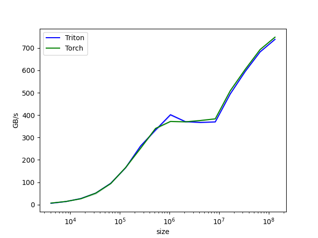 下面将实现一个融合的 softmax 操作,该操作在处理特定类型的矩阵时,性能显著优于 PyTorch 的原生实现。具体而言,当矩阵的行可以适应 GPU 的 SRAM 时,融合内核可以减少内存访问并提高计算效率。通过这个例子,我们将学习内核融合的好处以及 Triton 中的归约操作。
融合的 softmax实现示例代码如下:
"""
Fused Softmax
=============

In this tutorial, you will write a fused softmax operation that is significantly faster
than PyTorch's native op for a particular class of matrices: those whose rows can fit in
the GPU's SRAM.

In doing so, you will learn about:

* The benefits of kernel fusion for bandwidth-bound operations.

* Reduction operators in Triton.

"""

# %%
# Motivations
# -----------
#
# Custom GPU kernels for elementwise additions are educationally valuable but won't get you very far in practice.
# Let us consider instead the case of a simple (numerically stabilized) softmax operation:

import torch

import triton
import triton.language as tl
from triton.runtime import driver

def is_hip():
    return triton.runtime.driver.active.get_current_target().backend == "hip"

def is_cdna():
    return is_hip() and triton.runtime.driver.active.get_current_target().arch in ('gfx940', 'gfx941', 'gfx942',
                                                                                   'gfx90a', 'gfx908')

def naive_softmax(x):
    """Compute row-wise softmax of X using native pytorch

    We subtract the maximum element in order to avoid overflows. Softmax is invariant to
    this shift.
    """
    # read  MN elements ; write M  elements
    x_max = x.max(dim=1)[0]
    # read MN + M elements ; write MN elements
    z = x - x_max[:, None]
    # read  MN elements ; write MN elements
    numerator = torch.exp(z)
    # read  MN elements ; write M  elements
    denominator = numerator.sum(dim=1)
    # read MN + M elements ; write MN elements
    ret = numerator / denominator[:, None]
    # in total: read 5MN + 2M elements ; wrote 3MN + 2M elements
    return ret

# %%
# When implemented naively in PyTorch, computing :code:`y = naive_softmax(x)` for :math:`x \in R^{M \times N}`
# requires reading :math:`5MN + 2M` elements from DRAM and writing back :math:`3MN + 2M` elements.
# This is obviously wasteful; we'd prefer to have a custom "fused" kernel that only reads
# X once and does all the necessary computations on-chip.
# Doing so would require reading and writing back only :math:`MN` bytes, so we could
# expect a theoretical speed-up of ~4x (i.e., :math:`(8MN + 4M) / 2MN`).
# The `torch.jit.script` flags aims to perform this kind of "kernel fusion" automatically
# but, as we will see later, it is still far from ideal.

# %%
# Compute Kernel
# --------------
#
# Our softmax kernel works as follows: each program loads a set of rows of the input matrix X strided by number of programs,
# normalizes it and writes back the result to the output Y.
#
# Note that one important limitation of Triton is that each block must have a
# power-of-two number of elements, so we need to internally "pad" each row and guard the
# memory operations properly if we want to handle any possible input shapes:


@triton.jit
def softmax_kernel(output_ptr, input_ptr, input_row_stride, output_row_stride, n_rows, n_cols, BLOCK_SIZE: tl.constexpr,
                   num_stages: tl.constexpr):
    # starting row of the program
    row_start = tl.program_id(0)
    row_step = tl.num_programs(0)
    for row_idx in tl.range(row_start, n_rows, row_step, num_stages=num_stages):
        # The stride represents how much we need to increase the pointer to advance 1 row
        row_start_ptr = input_ptr + row_idx * input_row_stride
        # The block size is the next power of two greater than n_cols, so we can fit each
        # row in a single block
        col_offsets = tl.arange(0, BLOCK_SIZE)
        input_ptrs = row_start_ptr + col_offsets
        # Load the row into SRAM, using a mask since BLOCK_SIZE may be > than n_cols
        mask = col_offsets < n_cols
        row = tl.load(input_ptrs, mask=mask, other=-float('inf'))
        # Subtract maximum for numerical stability
        row_minus_max = row - tl.max(row, axis=0)
        # Note that exponentiation in Triton is fast but approximate (i.e., think __expf in CUDA)
        numerator = tl.exp(row_minus_max)
        denominator = tl.sum(numerator, axis=0)
        softmax_output = numerator / denominator
        # Write back output to DRAM
        output_row_start_ptr = output_ptr + row_idx * output_row_stride
        output_ptrs = output_row_start_ptr + col_offsets
        tl.store(output_ptrs, softmax_output, mask=mask)

# %%
# We can create a helper function that enqueues the kernel and its (meta-)arguments for any given input tensor.

device = torch.cuda.current_device()
properties = driver.active.utils.get_device_properties(device)
NUM_SM = properties["multiprocessor_count"]
NUM_REGS = properties["max_num_regs"]
SIZE_SMEM = properties["max_shared_mem"]
WARP_SIZE = properties["warpSize"]
target = triton.runtime.driver.active.get_current_target()
kernels = {}


def softmax(x):
    n_rows, n_cols = x.shape

    # The block size of each loop iteration is the smallest power of two greater than the number of columns in `x`
    BLOCK_SIZE = triton.next_power_of_2(n_cols)

    # Another trick we can use is to ask the compiler to use more threads per row by
    # increasing the number of warps (`num_warps`) over which each row is distributed.
    # You will see in the next tutorial how to auto-tune this value in a more natural
    # way so you don't have to come up with manual heuristics yourself.
    num_warps = 8

    # Number of software piepling stages.
    num_stages = 4 if SIZE_SMEM > 200000 else 2

    # Allocate output
    y = torch.empty_like(x)

    # pre-compile kernel to get register usage and compute thread occupancy.
    kernel, num_programs = kernels.get(BLOCK_SIZE, (None, 0))
    if kernel is None:
        kernel = softmax_kernel.warmup(y, x, x.stride(0), y.stride(0), n_rows, n_cols, BLOCK_SIZE=BLOCK_SIZE,
                                       num_stages=num_stages, num_warps=num_warps, grid=(1, ))
        kernel._init_handles()
        n_regs = kernel.n_regs
        size_smem = kernel.metadata.shared
        if is_hip():
            # NUM_REGS represents the number of regular purpose registers. On CDNA architectures this is half of all registers available.
            # However, this is not always the case. In most cases all registers can be used as regular purpose registers.
            # ISA SECTION (3.6.4 for CDNA3)
            # VGPRs are allocated out of two pools: regular VGPRs and accumulation VGPRs. Accumulation VGPRs are used
            # with matrix VALU instructions, and can also be loaded directly from memory. A wave may have up to 512 total
            # VGPRs, 256 of each type. When a wave has fewer than 512 total VGPRs, the number of each type is flexible - it is
            # not required to be equal numbers of both types.
            if is_cdna():
                NUM_GPRS = NUM_REGS * 2

            # MAX_NUM_THREADS represents maximum number of resident threads per multi-processor.
            # When we divide this number with WARP_SIZE we get maximum number of waves that can
            # execute on a CU (multi-processor)  in parallel.
            MAX_NUM_THREADS = properties["max_threads_per_sm"]
            max_num_waves = MAX_NUM_THREADS // WARP_SIZE
            occupancy = min(NUM_GPRS // WARP_SIZE // n_regs, max_num_waves) // num_warps
        else:
            occupancy = NUM_REGS // (n_regs * WARP_SIZE * num_warps)
        occupancy = min(occupancy, SIZE_SMEM // size_smem)
        num_programs = NUM_SM * occupancy
        kernels[BLOCK_SIZE] = (kernel, num_programs)

    num_programs = min(num_programs, n_rows)

    # Create a number of persistent programs.
    kernel[(num_programs, 1, 1)](
        y,
        x,
        x.stride(0),
        y.stride(0),
        n_rows,
        n_cols,
    )
    return y

# %%
# Unit Test
# ---------

# %%
# We make sure that we test our kernel on a matrix with an irregular number of rows and columns.
# This will allow us to verify that our padding mechanism works.

torch.manual_seed(0)
x = torch.randn(1823, 781, device='cuda')
y_triton = softmax(x)
y_torch = torch.softmax(x, axis=1)
assert torch.allclose(y_triton, y_torch), (y_triton, y_torch)

# %%
# As expected, the results are identical.

# %%
# Benchmark
# ---------
#
# Here we will benchmark our operation as a function of the number of columns in the input matrix -- assuming 4096 rows.
# We will then compare its performance against (1) :code:`torch.softmax` and (2) the :code:`naive_softmax` defined above.


@triton.testing.perf_report(
    triton.testing.Benchmark(
        x_names=['N'],  # argument names to use as an x-axis for the plot
        x_vals=[128 * i for i in range(2, 100)],  # different possible values for `x_name`
        line_arg='provider',  # argument name whose value corresponds to a different line in the plot
        line_vals=['triton', 'torch'],  # possible values for `line_arg``
        line_names=[
            "Triton",
            "Torch",
        ],  # label name for the lines
        styles=[('blue', '-'), ('green', '-')],  # line styles
        ylabel="GB/s",  # label name for the y-axis
        plot_name="softmax-performance",  # name for the plot. Used also as a file name for saving the plot.
        args={'M': 4096},  # values for function arguments not in `x_names` and `y_name`
    ))
def benchmark(M, N, provider):
    x = torch.randn(M, N, device='cuda', dtype=torch.float32)
    stream = torch.cuda.Stream()
    torch.cuda.set_stream(stream)
    if provider == 'torch':
        ms = triton.testing.do_bench(lambda: torch.softmax(x, axis=-1))
    if provider == 'triton':
        ms = triton.testing.do_bench(lambda: softmax(x))
    gbps = lambda ms: 2 * x.nelement() * x.element_size() * 1e-9 / (ms * 1e-3)
    return gbps(ms)

benchmark.run(show_plots=True, print_data=True, save_path="output")
结果:
softmax-performance:
          N      Triton       Torch
0     256.0  286.304086  374.914120
1     384.0  334.484465  371.506107
2     512.0  409.811791  299.262763
3     640.0  380.141194  320.723956
4     768.0  387.645576  304.382499
5     896.0  373.444696  292.122508
6    1024.0  359.742054  292.430046
7    1152.0  364.509882  440.223322
...
96  12544.0  626.395424  620.854101
97  12672.0  628.975394  642.458547
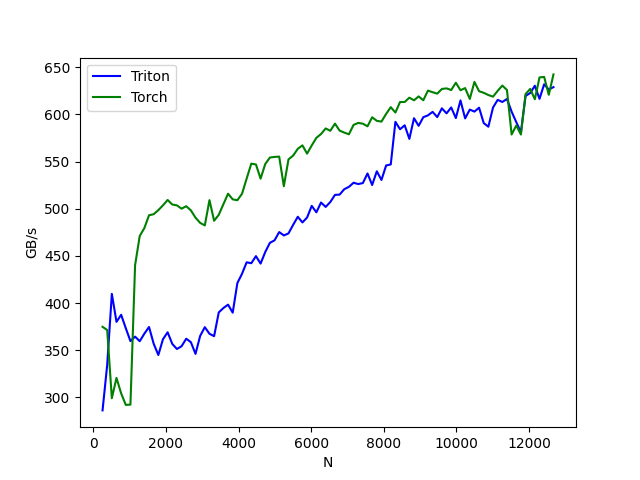
矩阵乘法的实现示例代码如下:
import torch
import triton
import triton.language as tl
import time

# Define matrix multiplication kernel using Triton
@triton.jit
def matmul_kernel(
    A, B, C, M, N, K, BLOCK_M: tl.constexpr, BLOCK_N: tl.constexpr, BLOCK_K: tl.constexpr,
):
    pid = tl.program_id(0)
    row = pid // (N // BLOCK_N)
    col = pid % (N // BLOCK_N)

    offs_m = row * BLOCK_M + tl.arange(0, BLOCK_M)
    offs_n = col * BLOCK_N + tl.arange(0, BLOCK_N)
    offs_k = tl.arange(0, BLOCK_K)

    a_ptrs = A + offs_m[:, None] * K + offs_k[None, :]
    b_ptrs = B + offs_k[:, None] * N + offs_n[None, :]

    accum = tl.zeros((BLOCK_M, BLOCK_N), dtype=tl.float32)

    for k in range(0, K, BLOCK_K):
        a = tl.load(a_ptrs)
        b = tl.load(b_ptrs)
        accum += tl.dot(a, b)
        a_ptrs += BLOCK_K
        b_ptrs += BLOCK_K * N

    c_ptrs = C + offs_m[:, None] * N + offs_n[None, :]
    tl.store(c_ptrs, accum)

def matmul(a, b):
    num_iters = 300
    M, K = a.shape
    N = b.shape[1]
    C = torch.zeros((M, N), dtype=torch.float32, device='cuda')

    # Compile and run Triton kernel
    grid = (M // 32, N // 32)

    start = time.time()
    print("[Matrix Multiply Using Triton] - Starting...")
    print(f"MatrixA({M},{K}), MatrixB({K},{N})")

    for _ in range(num_iters):
        matmul_kernel[grid](a, b, C, M, N, K, BLOCK_M=32, BLOCK_N=32, BLOCK_K=32)

    torch.cuda.synchronize()
    end = time.time()

    # Calculate performance metrics
    elapsed_time = end - start
    time_per_iteration = elapsed_time * 1000 / num_iters
    flops = 2.0 * M * N * K * num_iters
    gflops = (flops / elapsed_time) / 1e9

    # Output performance results
    print(f"Triton Performance= {gflops:.2f} GFlop/s, Time= {time_per_iteration:.3f} msec")
    return C

# Matrix sizes
M, N, K = 320, 320, 320

# Initialize matrices
A = torch.randn((M, K), dtype=torch.float16, device='cuda')
B = torch.randn((K, N), dtype=torch.float16, device='cuda')

# Call the matmul function
C = matmul(A, B)
print(f"Output matrix C: {C}")
结果:
[Matrix Multiply Using Triton] - Starting...
MatrixA(320,320), MatrixB(320,320)
Triton Performance= 52.65 GFlop/s, Time= 1.245 msec
Output matrix C: tensor([[ 20.6646,  -1.4497,   1.6400,  ...,  11.9098,  12.1640, -13.7652],
        [ 10.9663,  -3.8929,  12.4444,  ...,  -9.7939, -19.5267, -21.4840],
        [  1.5969,  -0.4670,  48.2527,  ..., -18.8371,  22.3166, -23.5707],
        ...,
        [  0.0000,   0.0000,   0.0000,  ...,   0.0000,   0.0000,   0.0000],
        [  0.0000,   0.0000,   0.0000,  ...,   0.0000,   0.0000,   0.0000],
        [  0.0000,   0.0000,   0.0000,  ...,   0.0000,   0.0000,   0.0000]],
       device='cuda:0')
框架模型层(同chapter3.4 6)
Triton 可以与 PyTorch 框架无缝集成,虽然 PyTorch 模型不会直接转换为 Triton,但可以利用 Triton 编写自定义的 CUDA 核心,从而优化特定的操作。这种方式让开发者可以在 PyTorch 中使用 Triton 优化的操作,提升性能。
例如,在 PyTorch 模型中包装 Triton 核心的代码:
class MyModel(torch.nn.Module):
    def forward(self, x, y):
        z = triton_add_wrapper(x, y)
        return z
Unsloth 是一个高效的库,使用 Triton 编写的算子,能够实现高性能的模型训练和推理,且没有准确性损失。下面是使用 Unsloth 的 FastLanguageModel 来加载一个预训练的 LLaMA 3 模型并进行推理的示例代码:
import time
import torch
from unsloth import FastLanguageModel

max_seq_length = 2048 # Choose any! We auto support RoPE Scaling internally!
dtype = None # None for auto detection. Float16 for Tesla T4, V100, Bfloat16 for Ampere+
load_in_4bit = True # Use 4bit quantization to reduce memory usage. Can be False.

model, tokenizer = FastLanguageModel.from_pretrained(
    model_name = "/home/aii-works/llama3/Meta-Llama-3-8B-Instruct",
    max_seq_length = max_seq_length,
    dtype = dtype,
    load_in_4bit = load_in_4bit
)

model = FastLanguageModel.get_peft_model(
    model,
    r = 16, # Choose any number > 0 ! Suggested 8, 16, 32, 64, 128
    target_modules = ["q_proj", "k_proj", "v_proj", "o_proj",
                      "gate_proj", "up_proj", "down_proj",],
    lora_alpha = 16,
    lora_dropout = 0, # Supports any, but = 0 is optimized
    bias = "none",    # Supports any, but = "none" is optimized
    # [NEW] "unsloth" uses 30% less VRAM, fits 2x larger batch sizes!
    use_gradient_checkpointing = "unsloth", # True or "unsloth" for very long context
    random_state = 3407,
    use_rslora = False,  # We support rank stabilized LoRA
    loftq_config = None, # And LoftQ
)

alpaca_prompt = """Below is an instruction that describes a task, paired with an input that provides further context. Write a response that appropriately completes the request.

### Instruction:
{}

### Input:
{}

### Response:
{}"""

FastLanguageModel.for_inference(model)

inputs = tokenizer(
[
    alpaca_prompt.format(
        # "Continue the fibonnaci sequence.", # instruction
        "Q:",
        "Name the planets in the solar system?",
        "", # output - leave this blank for generation!
    )
], return_tensors = "pt").to("cuda")

iterations = 10
with torch.no_grad():
    for _ in range(5):
        outputs = model.generate(**inputs, max_new_tokens = 64, use_cache = True)
t_start = time.time()
for _ in range(iterations):
    with torch.no_grad():
        outputs = model.generate(**inputs, max_new_tokens = 64, use_cache = True)
elapsed_time = time.time() - t_start
latency = elapsed_time / iterations * 1000
FPS = 1000 / latency

print(tokenizer.decode(outputs[0], skip_special_tokens=True))
print(f"FPS: {FPS:.2f}")
结果:
🦥 Unsloth: Will patch your computer to enable 2x faster free finetuning.
==((====))==  Unsloth 2024.8: Fast Llama patching. Transformers = 4.44.2.
   \\   /|    GPU: NVIDIA GeForce RTX 4080 SUPER. Max memory: 15.695 GB. Platform = Linux.
O^O/ \_/ \    Pytorch: 2.4.0. CUDA = 8.9. CUDA Toolkit = 12.1.
\        /    Bfloat16 = TRUE. FA [Xformers = 0.0.27.post2. FA2 = False]
 "-____-"     Free Apache license: http://github.com/unslothai/unsloth
Loading checkpoint shards: 100%|███████████████████████████████████████████████████████████████████████████████████████████████████████████████████████████████████████████████████████████████████████| 4/4 [00:02<00:00,  1.76it/s]
/home/aii-works/llama3/Meta-Llama-3-8B-Instruct does not have a padding token! Will use pad_token = <|reserved_special_token_250|>.
Unsloth 2024.8 patched 32 layers with 32 QKV layers, 32 O layers and 32 MLP layers.
huggingface/tokenizers: The current process just got forked, after parallelism has already been used. Disabling parallelism to avoid deadlocks...
To disable this warning, you can either:
        - Avoid using `tokenizers` before the fork if possible
        - Explicitly set the environment variable TOKENIZERS_PARALLELISM=(true | false)
huggingface/tokenizers: The current process just got forked, after parallelism has already been used. Disabling parallelism to avoid deadlocks...
To disable this warning, you can either:
        - Avoid using `tokenizers` before the fork if possible
        - Explicitly set the environment variable TOKENIZERS_PARALLELISM=(true | false)
Below is an instruction that describes a task, paired with an input that provides further context. Write a response that appropriately completes the request.

### Instruction:
Q:

### Input:
Name the planets in the solar system?

### Response:
The eight planets in our solar system, in order from the Sun, are:

1. Mercury
2. Venus
3. Earth
4. Mars
5. Jupiter
6. Saturn
7. Uranus
8. Neptune

Note: Pluto was previously considered a planet, but in 2006,
FPS: 0.89
Apache TVM (AMD)
TVM 支持的硬件概述 下图显示了 TVM 当前支持的硬件后端:
技术栈架构
NVIDIA 平台:基于 CUDA 的技术栈架构高度集成,提供了丰富的硬件加速功能,如 Tensor Cores,以及深度优化的库(cuBLAS、cuDNN、TensorRT),使得 TVM 能够通过多层次优化,充分发挥 NVIDIA GPU 的潜力,适用于大规模深度学习训练和推理任务。
AMD 平台:ROCm 提供了开放的技术栈,结合 HIP 编程模型,使得 TVM 能够在 AMD GPU 上运行。但与 NVIDIA 的专有技术栈相比,AMD 平台的硬件加速支持较少,库优化较为基础,导致 TVM 在 AMD GPU 上的性能表现不如 NVIDIA 平台强劲。AMD 在异构计算和跨平台兼容性方面表现更好,但在深度学习推理任务中,其优化深度仍有待提高。
系统软件层
TVM 与 AMD GPU 通过 ROCm 进行交互的完整流程:
-
初始化 GPU 上下文:使用
hipSetDevice(device_id)选择特定的 GPU 设备。这一步确保后续操作在正确的 GPU 上执行。 -
分配 GPU 显存:调用
hipMalloc(&device_ptr, size)来在 GPU 上分配所需的显存。这将为输入、输出和中间计算结果分配空间。若不再需要这些显存,可以使用hipFree(device_ptr)释放显存,以防内存泄漏。 -
数据传输:使用
hipMemcpy(device_ptr, host_ptr, size, hipMemcpyHostToDevice)将数据从主机(CPU)传输到设备(GPU)。当 GPU 计算完成后,通过hipMemcpy(host_ptr, device_ptr, size, hipMemcpyDeviceToHost)将结果从设备传回主机。 -
加载和执行内核:使用
hipModuleLoad(&module, "kernel_name")加载 CUDA 内核模块。通过hipModuleGetFunction(&function, module, "kernel_function_name")获取内核函数句柄。配置线程块和线程网格后,使用hipLaunchKernel(function, grid_dim, block_dim, args, shared_mem_size, stream)启动内核。 -
同步 GPU 操作:使用
hipDeviceSynchronize()确保所有发起的 GPU 操作都已完成。这一步是必要的,以保证主机在继续执行后续操作时能获取正确的结果。 -
释放资源:在计算任务完成后,使用
hipFree(device_ptr)释放显存,并使用hipModuleUnload(module)卸载内核模块,确保没有资源泄漏。
运行时环境层
通过 TVM 来检查是否支持 ROCm 设备(Radeon Open Compute),并输出设备的相关信息。
- 函数 check_rocm 用于检查当前是否有可用的 ROCm 设备。 tvm.runtime.device("rocm", 0) 用于获取第 0 个 ROCm 设备(设备 ID 为 0),并返回一个设备对象。
- device.exist 用于检查获取的设备是否存在。如果设备不可用(device.exist 为 False),则输出 "ROCm 设备不可用" 并返回 None,表示没有找到可用的 ROCm 设备。
- 调用 check_rocm 函数并将返回值赋给变量 device。如果 device 为 None,说明没有可用的 ROCm 设备。
- 如果设备存在(device 不为 None),则创建一个 device_info 字典,包含设备的类型 (device.device_type) 和设备 ID (device.device_id)。 device.device_type: 返回设备的类型,这里应该是 "rocm"。 device.device_id: 返回设备的 ID,这里应该是 0,因为设备是通过 tvm.runtime.device("rocm", 0) 获取的。
代码:
import tvm

# 检查 TVM 是否支持 ROCm 并返回设备详细信息
def check_rocm():
    try:
        # 获取 ROCm 设备
        device = tvm.runtime.device("rocm", 0)

        # 检查设备是否可用
        if not device.exist:
            print("ROCm 设备不可用")
            return None

        print("ROCm check success")
        return device
    except Exception as e:
        print(f"ROCm check failed: {e}")
        return None

device = check_rocm()

# 获取当前可用的设备并输出设备信息
if device:
    device_info = {
        "device_type": device.device_type,
        "device_id": device.device_id
    }
    print("Device Info:")
    for key, value in device_info.items():
        print(f"  {key}: {value}")
结果:
ROCm check success
Device Info:
  device_type: rocm
  device_id: 0
编程模型和语言层
运行过程与结果与NV相同
TVM 是一个专注于深度学习模型优化和编译的开源框架,它的编程模型基于 Tensor 表达、算子(Operator)定义 和 调度(Schedule),并且通过高效代码生成实现硬件上的高性能计算。TVM 编程模型的关键步骤包括:
- 定义计算:使用 TVM 的计算表达式定义要执行的计算任务。
- 调度(Scheduling):为计算任务安排执行顺序和资源分配,指定如何并行化、向量化等。
- 编译:将计算和调度方案编译为可在目标硬件上运行的代码。
- 执行:在目标设备上运行编译后的代码。
下面是一个简单的示例,它展示了TVM的基本编程流程,包括定义矩阵加法运算并在CPU或者GPU上执行。
TVM 的编程模型示例
import tvm
from tvm import te
import numpy as np

# 1. 定义计算:A 和 B 矩阵相加,生成 C
n = te.var("n")
A = te.placeholder((n,), name="A")
B = te.placeholder((n,), name="B")
C = te.compute(A.shape, lambda i: A[i] + B[i], name="C")

# 2. 创建调度:默认调度会按顺序执行计算
s = te.create_schedule(C.op)

# 3. 编译:为 GPU 生成低级代码
target = "llvm"  # CPU 目标 如果是hi是GPU上执行则改为“cuda”
fadd = tvm.build(s, [A, B, C], target, name="matrix_add")

# 4. 在 TVM 运行时中执行
ctx = tvm.cpu(0)
n_value = 1024
a = tvm.nd.array(np.random.uniform(size=n_value).astype(A.dtype), ctx)
b = tvm.nd.array(np.random.uniform(size=n_value).astype(B.dtype), ctx)
c = tvm.nd.array(np.zeros(n_value, dtype=C.dtype), ctx)

# 调用编译好的函数
fadd(a, b, c)

# 检查结果
np.testing.assert_allclose(c.asnumpy(), a.asnumpy() + b.asnumpy())
print("Result matches with NumPy calculation.")
代码解释
-
定义计算:
- 使用
te.placeholder创建两个占位符A和B,分别代表输入的矩阵。 - 使用
te.compute定义计算表达式,这里表示逐元素对A和B执行加法操作,结果存储在C中。
- 使用
-
调度计算:
- 使用
te.create_schedule(C.op)创建调度。这里使用的是默认的顺序执行调度,也可以通过优化调度提升性能。
- 使用
-
编译代码:
- 使用
tvm.build函数,将计算和调度编译成针对指定目标(如 CPU 或 GPU)的可执行代码。
- 使用
-
运行并验证结果:
- 创建 TVM 的
nd.array将 NumPy 数据传入 TVM 中运行。 - 使用编译好的函数
fadd进行计算,并验证结果是否与 NumPy 计算的结果一致。 结果
- 创建 TVM 的
Result matches with NumPy calculation.
这个简单的例子展示了 TVM 的核心编程流程。在实际的深度学习模型优化中,TVM 提供了更多高级特性,例如自动调度(AutoScheduler)、多目标硬件支持(CPU、GPU、TPU)等,可以极大提升模型在不同硬件平台上的运行效率。
下面再给一个 TVM 示例,这次展示如何使用 TVM 优化二维矩阵乘法(矩阵乘法是深度学习中常见的操作之一),并进行简单的调度优化。
TVM 矩阵乘法示例
import tvm
from tvm import te
import numpy as np

# 1. 定义矩阵乘法计算: C[i, j] = sum(A[i, k] * B[k, j] for k in range(K))
N = te.var("N")
M = te.var("M")
K = te.var("K")

# 定义矩阵 A, B
A = te.placeholder((N, K), name="A")
B = te.placeholder((K, M), name="B")

# 定义矩阵乘法的计算
C = te.compute((N, M), lambda i, j: te.sum(A[i, k] * B[k, j] for k in range(K)), name="C")

# 2. 创建调度
s = te.create_schedule(C.op)

# 简单调度优化:并行化行方向上的计算
# 这是 TVM 调度中常见的优化方式
s[C].parallel(C.op.axis[0])

# 3. 编译:为 CPU 生成代码
target = "llvm"  # CPU 目标
fmatmul = tvm.build(s, [A, B, C], target, name="matrix_multiply")

# 4. 在 TVM 运行时中执行
ctx = tvm.cpu(0)

# 定义矩阵的大小
N_value = 1024
M_value = 1024
K_value = 1024

# 创建随机的输入矩阵 A 和 B
a = tvm.nd.array(np.random.uniform(size=(N_value, K_value)).astype(A.dtype), ctx)
b = tvm.nd.array(np.random.uniform(size=(K_value, M_value)).astype(B.dtype), ctx)
c = tvm.nd.array(np.zeros((N_value, M_value), dtype=C.dtype), ctx)

# 调用编译好的矩阵乘法函数
fmatmul(a, b, c)

# 使用 NumPy 计算参考结果
np_c = np.dot(a.asnumpy(), b.asnumpy())

# 验证 TVM 计算的结果是否与 NumPy 的结果一致
np.testing.assert_allclose(c.asnumpy(), np_c, rtol=1e-5)
print("Matrix multiplication result matches with NumPy.")
代码解释
-
定义矩阵乘法:
- 使用
te.placeholder创建两个占位符A和B,分别代表输入的二维矩阵。 - 使用
te.compute定义矩阵乘法,te.sum用于对中间维度K进行求和,从而实现矩阵乘法的核心计算。
- 使用
-
调度优化:
- 使用
te.create_schedule(C.op)创建调度方案。 - 通过
s[C].parallel(C.op.axis[0])让 TVM 并行化行方向上的计算,这是一个简单的优化方法,用于利用多核 CPU 提升矩阵乘法的性能。
- 使用
-
编译代码:
- 使用
tvm.build将计算和调度方案编译成可执行的 CPU 代码。
- 使用
-
运行并验证结果:
- 创建随机的矩阵
A和B,在 TVM 的运行时环境中执行编译好的矩阵乘法函数。 - 使用 NumPy 的
dot函数计算参考矩阵乘法的结果,并与 TVM 的结果进行比较,确保其一致性。
- 创建随机的矩阵
结果
Matrix multiplication result matches with NumPy.
这表明 TVM 编译后的矩阵乘法操作正确地执行,并且与 NumPy 的计算结果一致。
计算库层
运行过程与结果与NV相同
TVM 仓库的根目录包含以下几个子目录:
- src:存放用于算子编译和部署运行时的 C++ 代码。
- src/relay:实现了 Relay,这是一个为深度学习框架提供的新功能 IR。
- python:提供 Python 前端,用于封装 src 中实现的 C++ 函数和对象。
- src/topi:定义标准神经网络算子的计算和后端调度。
src/relay 是负责管理计算图的组件,其中图结构中的节点通过 src 其余部分提供的基础设施进行编译和执行。python 为 C++ API 和执行编译的驱动代码提供了 Python 绑定。与节点对应的算子在 src/relay/op 中注册,而算子的实现则在 topi 中,使用的编程语言包括 C++ 和 Python。
其中:
- IR(Intermediate Representation):一种中间表示形式,用于编译过程中的高级代码表示。
- 算子(Operator):在深度学习中,算子通常指代执行特定计算的函数,比如卷积、矩阵乘等。
- 调度(Schedule):定义了算子如何在硬件上执行的策略,包括循环的嵌套结构、并行化、向量化等。
向量加法示例:
n = 1024
A = tvm.te.placeholder((n,), name='A')
B = tvm.te.placeholder((n,), name='B')
C = tvm.te.compute(A.shape, lambda i: A[i] + B[i], name="C")
在 python/tvm/te/tensor.py 中定义的 A、B 和 C 的类型都是 tvm.tensor.Tensor。这些 Python Tensor 是由 C++ Tensor 支持的,其实现位于 include/tvm/te/tensor.h 和 src/te/tensor.cc 文件中。在 TVM 中,所有的 Python 类型都可以视为与其底层 C++ 类型具有相同名称的句柄。
从以下 Python Tensor 类型的定义中可以看出,tvm.tensor.Tensor 是 Object 的一个子类。
@register_object
class Tensor(Object, _expr.ExprOp):
    """Tensor object, to construct, see function.Tensor"""

    def __call__(self, *indices):
       ...
-
在 TVM 中,每个
Tensor对象都有一个与之关联的Operation对象。Tensor是在计算过程中存储数据的多维数组,而Operation表示对一个或多个Tensor进行操作的计算。这两个概念在代码中有明确的实现,相关定义分别在python/tvm/te/tensor.py、include/tvm/te/operation.h和src/tvm/te/operation目录下。 -
每个
Tensor对象都可以看作是其相应的Operation的输出,这意味着通过执行某个Operation可以生成一个Tensor。 -
Operation对象提供了一个input_tensors()方法,这个方法返回一个输入Tensor的列表。这使得开发者能够跟踪不同Operation之间的依赖关系,了解一个Operation需要哪些输入Tensor,以及这些输入Tensor是由哪些其他Operation产生的。 -
在计算图中,当我们想要调度某个计算时,需要将输出张量(例如上面提到的
C张量)对应的Operation对象传递给python/tvm/te/schedule.py中的tvm.te.create_schedule()函数create_schedule()函数负责生成计算的调度策略,以优化计算的执行。这是构建高效计算图的重要步骤,因为它允许对计算的执行顺序和方式进行控制,从而提高性能。
S = tvm.te.create_schedule(C.op)
函数被映射到 include/tvm/schedule.h 中的 C++ 函数。
inline Schedule create_schedule(Array<Operation> ops) {
    return Schedule(ops);
}
-
在 TVM 中,调度由多个
Stage和输出的Operation组成。每个Stage代表一个Operation的计算过程。 -
以“向量加法”(Vector Add)为例,假设有两个占位符
Operation和一个计算Operation,那么这个调度(s)将包含三个阶段(Stage)。 -
每个
Stage存储有关循环嵌套的信息,包括:循环嵌套结构:描述了如何将计算划分为多个循环的结构。循环类型:标识每个循环的执行方式,比如:Parallel(并行):表示该循环可以在多个线程中并行执行。Vectorized(向量化):表示该循环将数据分块处理,以提高效率。Unrolled(展开):表示将循环展开为多个相同的操作,以减少循环开销。位置:指明在下一个Stage的循环嵌套中执行该计算的位置(如果有嵌套的话)。create_schedule() 函数的作用:create_schedule()函数用于创建默认的调度。这个调度提供了基础的计算顺序和结构。默认的调度通常会调用tvm.build(...)函数来生成可执行的代码。 -
为了使调度可以在 GPU 上运行,需要为调度中的
Stage绑定必要的线程。这一步骤是非常重要的,因为 GPU 的并行计算能力依赖于对线程的有效管理和分配。 -
通过线程绑定,开发者可以控制计算的并行性,从而充分利用 GPU 的硬件资源,以实现更高的性能。
target = "rocm"

# 分割轴,bx 和 tx 分别代表 block 和 thread
bx, tx = s[C].split(C.op.axis[0], factor=64)

# 将 bx 绑定到 blockIdx.x (表示块索引)
s[C].bind(bx, tvm.te.thread_axis("blockIdx.x"))

# 将 tx 绑定到 threadIdx.x (表示线程索引)
s[C].bind(tx, tvm.te.thread_axis("threadIdx.x"))

# 构建函数,目标平台为 ROCm
fadd = tvm.build(s, [A, B, C], target)
- 将目标 target 从 "cuda" 修改为 "rocm",这是 AMD GPU 上 TVM 使用的编译目标。 线程和块绑定:TVM 的线程绑定方式与 CUDA 类似,所以 thread_axis("blockIdx.x") 和 thread_axis("threadIdx.x") 不需要修改,它们仍然表示块索引和线程索引,适用于 rocm。
split和bind是调度操作,用于优化并行执行。split将计算操作的循环分割成更小的部分,bind将这些分割的部分绑定到GPU的线程和块上。tvm.build函数接受调度、输入和输出Tensor以及目标平台,然后返回一个可以在该平台上运行的模块。
tvm.build() 函数:
-
tvm.build()函数定义在python/tvm/driver/build_module.py中。它的主要作用是接收一个调度(schedule)、输入和输出的Tensor,以及一个目标设备(target),然后返回一个tvm.runtime.Module对象。返回的tvm.runtime.Module对象包含一个可以通过函数调用的已编译函数,这意味着用户可以直接调用这个编译后的函数进行计算,而无需关心底层实现细节。 -
tvm.build()的过程可以分为两个主要步骤:降级:降级过程将高级、初始的循环嵌套结构转化为最终的底层中间表示(IR)。这一过程是由tvm.lower()函数完成的,tvm.lower()也定义在python/tvm/build_module.py中。降级的第一步是进行边界推断,确定每个循环的迭代范围,以便在生成 IR 时确保计算的正确性。随后,tvm.lower()会创建一个初始的循环嵌套结构,以便更好地表达计算的逻辑和顺序。代码生成:在降级完成后,接下来的步骤是根据底层的 IR 生成目标机器代码。这一过程涉及将 IR 转换为特定硬件可以理解和执行的机器代码。 -
降级的过程有助于将更高级的计算抽象(例如高层的循环结构和调度策略)转化为更为底层的表示,使得后续的代码生成过程能够更加有效地针对特定硬件进行优化。通过将计算表示降级到 IR,TVM 能够更灵活地进行优化并适配多种硬件目标
def lower(sch,
          args,
          name="default_function",
          binds=None,
          simple_mode=False):
   ...
   bounds = schedule.InferBound(sch)
   stmt = schedule.ScheduleOps(sch, bounds)
   ...
边界推断(Bound Inference):
- 边界推断是一个关键的过程,它用于推断所有循环的边界和中间缓冲区的大小。这对于生成有效的代码和优化计算非常重要。
- 这一过程确保了在运行时可以有效利用共享内存,从而提高计算性能。
边界推断的实现:边界推断的实现代码位于以下文件中:
-
src/te/schedule/bound.cc -
src/te/schedule/graph.cc -
src/te/schedule/message_passing.cc -
这些实现文件负责具体的边界推断算法和逻辑,包括如何根据调度信息推断出循环的边界和缓冲区的大小。
ScheduleOps() 的作用:
stmt是ScheduleOps()函数的输出,表示一个初始的循环嵌套结构。这个结构是调度的基础,反映了计算中循环的组织方式。- 如果调度过程中已经应用了
reorder或split等原语,则stmt将反映这些变化,确保生成的初始循环结构与应用的调度操作一致。 ScheduleOps()函数的定义位于src/te/schedule/schedule_ops.cc中。
接下来,对 stmt 在 src/tir/pass 子目录下进行降级处理。
...
stmt = ir_pass.VectorizeLoop(stmt)
...
stmt = ir_pass.UnrollLoop(
    stmt,
    cfg.auto_unroll_max_step,
    cfg.auto_unroll_max_depth,
    cfg.auto_unroll_max_extent,
    cfg.unroll_explicit)
...
-
在降级完成后,
build()函数负责从降级后的函数生成特定目标的机器代码。这一步是将中间表示(IR)转化为实际可执行的代码。 -
ir_pass.VectorizeLoop 是 TVM 的一个 IR 变换函数,作用是将代码中的循环转换为 SIMD(单指令多数据)向量化指令,利用硬件的向量化指令集提升性能。
-
stmt:这是一个中间表示(IR)节点,表示代码的结构(通常是一个 For 循环)。VectorizeLoop 会在循环中找到可以向量化的部分,并进行优化。 结果:向量化后的 stmt 将包含硬件可以直接执行的向量指令,从而提高并行度和数据处理效率。
-
除了生成目标专用的机器代码,TVM 还会生成一段宿主机代码。这部分代码负责执行一些重要的任务,如内存管理和内核启动等。宿主机代码确保了生成的内核能够在目标设备上正确运行并管理资源。
-
代码生成的具体实现是在
build_module()函数中完成的,该函数定义在python/tvm/target/codegen.py中。这个 Python 函数负责协调代码生成的各个环节。 -
在 C++ 端,代码生成的实现细节位于
src/target/codegen子目录中。这里包含了许多与代码生成相关的实现和优化。 -
build_module()函数最终会调用 C++ 端的Build()函数,后者位于src/target/codegen/codegen.cc中。Build()函数负责将具体的代码生成逻辑实现,完成从中间表示到目标机器代码的转换。
TVM_REGISTER_GLOBAL("codegen.build_rocm")
.set_body([](TVMArgs args, TVMRetValue* rv) {
    *rv = BuildROCM(args[0]);  // 使用 BuildROCM 函数构建 ROCm 代码
});
-
将全局注册的名称从 "codegen.build_cuda" 改为 "codegen.build_rocm",表示这是针对 ROCm 的代码生成器。
-
将原来的 BuildCUDA 换为 BuildROCM,这个函数是 TVM 中处理 ROCm 代码生成的具体实现。
-
如果目标是使用 LLVM 后端(如 x86、ARM、NVPTX 和 AMDGPU),代码生成主要由定义在
src/codegen/llvm/codegen_llvm.cc中的CodeGenLLVM类完成。 -
CodeGenLLVM的作用是将 TVM 的 IR 转换为 LLVM 的 IR。这一步是重要的,因为 LLVM 提供了强大的优化和代码生成能力。 -
在生成 LLVM IR 后,
CodeGenLLVM会执行一些 LLVM 优化。这些优化可以提高生成代码的性能,利用 LLVM 的优化工具链来提升最终机器代码的执行效率。 -
最后,
CodeGenLLVM会生成适用于特定目标架构的机器代码,使得该代码可以在不同的硬件上高效运行。
框架模型层
运行过程与结果与NV相同
实现了一个使用tvm库进行矩阵乘法的程序。该程序在设备上执行矩阵乘法运算,并测量其性能。
- 包含必要的库和头文件,包括运行库和辅助函数
- 定义矩阵乘法的维度: 设置矩阵 (A) 的大小为 (320* 640),矩阵 (B) 的大小为 (640* 320)。
- 构建计算图:使用
te.placeholder定义输入矩阵 (A) 和 (B)。使用te.compute定义输出矩阵 (C) 的计算逻辑,利用te.sum进行矩阵乘法。 - 创建调度:使用
te.create_schedule创建调度,并为 GPU 设置线程和块的调度。使用s[C].split和s[C].bind将计算任务分配到不同的 GPU 线程和块。 - 构建和运行函数
build_and_run:编译计算图为可执行的函数,并为输入矩阵分配随机数据。在设备上分配内存,创建 TVM 数组。计算 FLOPs,并在循环中执行矩阵乘法多次以计时。 - 计算性能指标:计算总运行时间和每秒浮点运算次数 (GFLOPS),并输出结果。
- 执行代码: 调用
build_and_run函数在 GPU 上执行矩阵乘法,并打印计算图的简化模式。
代码:
import tvm
from tvm import te
import numpy as np
import time

# 定义矩阵乘法的大小
M = 320
N = 640
K = 320

# 定义矩阵乘法
A = te.placeholder((M, N), name='A')
B = te.placeholder((N, K), name='B')
k = te.reduce_axis((0, N), name='k')
C = te.compute((M, K), lambda i, j: te.sum(A[i, k] * B[k, j], axis=k), name='C')

# 创建调度
s = te.create_schedule(C.op)

# GPU 线程调度
block_x = te.thread_axis("blockIdx.x")
block_y = te.thread_axis("blockIdx.y")
thread_x = te.thread_axis("threadIdx.x")
thread_y = te.thread_axis("threadIdx.y")

# 为 GPU 添加块和线程的调度
bx, tx = s[C].split(C.op.axis[0], factor=32)
by, ty = s[C].split(C.op.axis[1], factor=32)
s[C].bind(bx, block_x)
s[C].bind(by, block_y)
s[C].bind(tx, thread_x)
s[C].bind(ty, thread_y)

# 定义函数
def build_and_run(target_device="rocm", num_repeats=300):
    # 编译
    target = tvm.target.Target(target_device)
    f = tvm.build(s, [A, B, C], target=target, name='matmul')

    # 创建输入数据
    a_np = np.random.uniform(-1, 1, size=(M, N)).astype(np.float32)
    b_np = np.random.uniform(-1, 1, size=(N, K)).astype(np.float32)
    c_np = np.zeros((M, K), dtype=np.float32)

    # 在设备上分配内存
    dev = tvm.device(target_device, 0)
    a_tvm = tvm.nd.array(a_np, dev)
    b_tvm = tvm.nd.array(b_np, dev)
    c_tvm = tvm.nd.array(c_np, dev)

    # 计算 FLOPs(2 * M * N * K)
    flops = 2 * M * N * K

    # 运行并计时
    start_time = time.time()
    for i in range(num_repeats):
        f(a_tvm, b_tvm, c_tvm)
    dev.sync()  # 保证所有计算都已完成
    end_time = time.time()

    # 计算总时间和 GFLOPS
    total_time = end_time - start_time
    gflops = (flops * num_repeats) / (total_time * 1e9)

    # 输出结果
    print(f"Execution on {target_device} completed in {total_time:.4f} seconds for {num_repeats} iterations.")
    print(f"FLOPs: {flops} per matrix multiplication")
    print(f"GFLOPS: {gflops:.2f} GFLOPS")

# 在 GPU 上执行
build_and_run(target_device="rocm")
结果:
Execution on rocm completed in 0.1786 seconds for 300 iterations.
FLOPs: 131072000 per matrix multiplication
GFLOPS: 220.18 GFLOPS
实现了一个使用 TVM 的Auto-scheduling 进行算子优化。
- 定义一个带有偏置加法的矩阵乘法。这里使用了 TVM 张量表达式语言中的标准操作。区别在于函数定义上方使用了
register_workload装饰器。该函数应返回输入/输出张量列表。通过这些张量,auto-scheduler 可以得到整个计算图。 - 定义函数后,可以为 auto_scheduler 创建要搜索的任务。为这个矩阵乘法指定了特定的参数,如这里是两个大小为 1024x1024 的矩阵乘法。然后创建一个 N=L=M=1024 和 dtype="float32" 的搜索任务
num_measure_trials表示搜索过程中可用的测试试验次数。用RecordToFile将测试记录记录到文件matmul.json中。测试记录可用于查询历史最佳、恢复搜索以及以后进行更多分析。- auto-scheduling 完成后,可将 schedule 降级来查看 IR。auto-scheduler 执行合适的优化,包括多级循环切分、布局转换、并行化、向量化、循环展开和算子融合。
代码:
import logging
import sys
import numpy as np
import tvm
from tvm import te
import tvm.testing

from tvm import autotvm
@auto_scheduler.register_workload  # Note the auto_scheduler decorator
def matmul_add(N, L, M, dtype):
    A = te.placeholder((N, L), name="A", dtype=dtype)
    B = te.placeholder((L, M), name="B", dtype=dtype)
    C = te.placeholder((N, M), name="C", dtype=dtype)

    k = te.reduce_axis((0, L), name="k")
    matmul = te.compute(
        (N, M),
        lambda i, j: te.sum(A[i, k] * B[k, j], axis=k),
        name="matmul",
        attrs={"layout_free_placeholders": [B]},  # enable automatic layout transform for tensor B
    )
    out = te.compute((N, M), lambda i, j: matmul[i, j] + C[i, j], name="out")

    return [A, B, C, out]
target = tvm.target.Target("llvm")
N = L = M = 1024
task = tvm.auto_scheduler.SearchTask(func=matmul_add, args=(N, L, M, "float32"), target=target)

# 检查计算图
print("Computational DAG:")
print(task.compute_dag)
log_file = "matmul.json"
tune_option = auto_scheduler.TuningOptions(
    num_measure_trials=10,
    measure_callbacks=[auto_scheduler.RecordToFile(log_file)],
    verbose=2,
)
# 运行 auto-tuning(搜索)
task.tune(tune_option)
# 应用最佳 schedule
sch, args = task.apply_best(log_file)
print("Lowered TIR:")
print(tvm.lower(sch, args, simple_mode=True))
结果:
Computational DAG:
A = PLACEHOLDER [1024, 1024]
B = PLACEHOLDER [1024, 1024]
matmul(i, j) += (A[i, k]*B[k, j])
C = PLACEHOLDER [1024, 1024]
out(i, j) = (matmul[i, j] + C[i, j])
Lowered TIR:
@main = primfn(A_1: handle, B_1: handle, C_1: handle, out_1: handle) -> ()
  attr = {"from_legacy_te_schedule": True, "global_symbol": "main", "tir.noalias": True}
  buffers = {A: Buffer(A_2: Pointer(float32), float32, [1048576], []),
             B: Buffer(B_2: Pointer(float32), float32, [1048576], []),
             C: Buffer(C_2: Pointer(float32), float32, [1048576], []),
             out: Buffer(out_2: Pointer(float32), float32, [1048576], [])}
  buffer_map = {A_1: A, B_1: B, C_1: C, out_1: out}
  preflattened_buffer_map = {A_1: A_3: Buffer(A_2, float32, [1024, 1024], []), B_1: B_3: Buffer(B_2, float32, [1024, 1024], []), C_1: C_3: Buffer(C_2, float32, [1024, 1024], []), out_1: out_3: Buffer(out_2, float32, [1024, 1024], [])} {
  allocate(auto_scheduler_layout_transform: Pointer(global float32), float32, [1048576]), storage_scope = global {
    for (ax0.ax1.fused.ax2.fused: int32, 0, 128) "parallel" {
      for (ax4: int32, 0, 256) {
        for (ax6: int32, 0, 4) {
          for (ax7: int32, 0, 8) {
            auto_scheduler_layout_transform_1: Buffer(auto_scheduler_layout_transform, float32, [1048576], [])[((((ax0.ax1.fused.ax2.fused*8192) + (ax4*32)) + (ax6*8)) + ax7)] = B[((((ax4*4096) + (ax6*1024)) + (ax0.ax1.fused.ax2.fused*8)) + ax7)]
          }
        }
      }
    }
    for (i.outer.outer.j.outer.outer.fused: int32, 0, 16384) "parallel" {
      allocate(matmul: Pointer(global float32x8), float32x8, [4]), storage_scope = global;
      for (i.outer.inner: int32, 0, 2) {
        matmul_1: Buffer(matmul, float32x8, [4], [])[0] = broadcast(0f32, 8)
        matmul_1[1] = broadcast(0f32, 8)
        matmul_1[2] = broadcast(0f32, 8)
        matmul_1[3] = broadcast(0f32, 8)
        for (k.outer: int32, 0, 256) {
          for (k.inner: int32, 0, 4) {
            let cse_var_2: int32 = (((floormod(i.outer.outer.j.outer.outer.fused, 128)*8192) + (k.outer*32)) + (k.inner*8))
            let cse_var_1: int32 = ((((floordiv(i.outer.outer.j.outer.outer.fused, 128)*8192) + (i.outer.inner*4096)) + (k.outer*4)) + k.inner)
             {
              matmul_1[0] = (matmul_1[0] + (broadcast(A[cse_var_1], 8)*auto_scheduler_layout_transform_1[ramp(cse_var_2, 1, 8)]))
              matmul_1[1] = (matmul_1[1] + (broadcast(A[(cse_var_1 + 1024)], 8)*auto_scheduler_layout_transform_1[ramp(cse_var_2, 1, 8)]))
              matmul_1[2] = (matmul_1[2] + (broadcast(A[(cse_var_1 + 2048)], 8)*auto_scheduler_layout_transform_1[ramp(cse_var_2, 1, 8)]))
              matmul_1[3] = (matmul_1[3] + (broadcast(A[(cse_var_1 + 3072)], 8)*auto_scheduler_layout_transform_1[ramp(cse_var_2, 1, 8)]))
            }
          }
        }
        for (i.inner: int32, 0, 4) {
          let cse_var_3: int32 = ((((floordiv(i.outer.outer.j.outer.outer.fused, 128)*8192) + (i.outer.inner*4096)) + (i.inner*1024)) + (floormod(i.outer.outer.j.outer.outer.fused, 128)*8))
          out[ramp(cse_var_3, 1, 8)] = (matmul_1[i.inner] + C[ramp(cse_var_3, 1, 8)])
        }
      }
    }
  }
}
实现了在 Relay 中定义神经网络,并为 GPU 生成 runtime 库。
- 使用 Relay 框架定义了 ResNet18 神经网络模型,设定批量大小为 1,图像形状为 (3, 224, 224),输出类别数为 1000。
- 输出 ResNet18 模型的计算图结构,
show_meta_data=False表示不显示元数据。 - 设置优化级别为 3(包括算子融合、预计算、布局变换等优化),并指定GPU作为目标设备,编译生成可在 GPU 上执行的库。
- 随机生成形状为
(1, 3, 224, 224)的输入数据。创建一个执行模块,并将输入数据设置到模型中,然后运行模型并获取输出结果。输出结果中的前 10 个元素。 - 使用 TVM 的
utils.tempdir创建临时目录,并将编译后的计算图、库和参数保存为文件,以便于后续部署时使用。 - 从保存的文件中加载编译模块,并使用相同的输入数据进行推理,获取输出结果。再次输出推理结果的前 10 个元素。
- 使用
tvm.testing.assert_allclose检查重新加载的模块输出与最初输出是否一致,容差设置为 1e-5。
import numpy as np
from tvm import relay
from tvm.relay import testing
import tvm
from tvm import te
from tvm.contrib import graph_executor
import tvm.testing

batch_size = 1
num_class = 1000
image_shape = (3, 224, 224)
data_shape = (batch_size,) + image_shape
out_shape = (batch_size, num_class)

# 获取 ResNet 模型
mod, params = relay.testing.resnet.get_workload(
    num_layers=18, batch_size=batch_size, image_shape=image_shape
)

# 为 AMD GPU (ROCm) 编译
opt_level = 3
target = tvm.target.rocm()  # 改为 rocm 目标
with tvm.transform.PassContext(opt_level=opt_level):
    lib = relay.build(mod, target, params=params)

# 创建图执行器,并在 AMD GPU 上运行该模块
# 创建随机输入
dev = tvm.rocm()  # 改为使用 ROCm 设备
data = np.random.uniform(-1, 1, size=data_shape).astype("float32")

# 创建模块
module = graph_executor.GraphModule(lib["default"](dev))

# 设置输入和参数
module.set_input("data", data)

# 运行
module.run()

# 获取输出
out = module.get_output(0, tvm.nd.empty(out_shape)).numpy()

# 打印输出的前 10 个元素
print(out.flatten()[0:10])
结果:
[0.00089283 0.00103331 0.0009094  0.00102275 0.00108751 0.00106737
 0.00106262 0.00095838 0.00110792 0.00113151]
# 创建随机输入
dev = tvm.rocm()  # 改为 ROCm 设备
data = np.random.uniform(-1, 1, size=data_shape).astype("float32")

# 创建图执行器模块
module = graph_executor.GraphModule(lib["default"](dev))

# 设置输入数据和参数
module.set_input("data", data)

# 在 AMD GPU 上运行
module.run()

# 获取输出
out = module.get_output(0, tvm.nd.empty(out_shape)).numpy()

# 打印输出的前 10 个元素
print(out.flatten()[0:10])
结果:
[0.00089283 0.00103331 0.0009094  0.00102275 0.00108751 0.00106737
 0.00106262 0.00095838 0.00110792 0.00113151]
# 保存和加载编译模块 分别将计算图、库和参数保存到不同文件

from tvm.contrib import utils

temp = utils.tempdir()
path_lib = temp.relpath("deploy_lib.tar")
lib.export_library(path_lib)
print(temp.listdir())

# 重新加载模块
loaded_lib = tvm.runtime.load_module(path_lib)
input_data = tvm.nd.array(data)
module = graph_executor.GraphModule(loaded_lib["default"](dev))
module.run(data=input_data)
out_deploy = module.get_output(0).numpy()

# 打印输出的前十个元素
print(out_deploy.flatten()[0:10])

# 检查来自部署模块的输出和原始输出是否一致
tvm.testing.assert_allclose(out_deploy, out, atol=1e-5)
结果:
['deploy_lib.tar']

[0.00089283 0.00103331 0.0009094  0.00102275 0.00108751 0.00106737
 0.00106262 0.00095838 0.00110792 0.00113151]
实现了将 ONNX 模型编译到 TVM Runtime并使用 TVMC 运行来自编译模块的模型
- 从指定的 URL 下载图像,并保存为
imagenet_cat.png。 - 使用 PIL 库将下载的图像大小调整为 224x224,以适应标准的图像输入要求(例如 ResNet)。
- 将图像数据从 HWC(Height-Width-Channel)格式转换为 NCHW(Channel-Height-Width)格式,这是 ONNX 模型的输入格式要求。
- 根据 ImageNet 的标准化方法,对图像进行归一化处理,减去均值
imagenet_mean并除以标准差imagenet_stddev。 - 将图像数据扩展一个维度,以符合神经网络模型所需的 batch 大小格式 (batch, channel, height, width)。
- 最终将预处理后的图像数据保存为
imagenet_cat.npz,用于后续推理。 - 从指定的 URL 下载 ImageNet 的类别标签列表,并保存为
synset.txt。 - 从保存的
predictions.npz文件中加载输出张量,该文件应是神经网络推理后的结果。 - 使用 softmax 函数将模型的输出转化为概率分布。根据概率分数对输出进行排序,选出排名前 5 的类别,并打印它们的标签及对应的概率。
from tvm.contrib.download import download_testdata
from PIL import Image
import numpy as np

img_url = "https://s3.amazonaws.com/model-server/inputs/kitten.jpg"
img_path = download_testdata(img_url, "imagenet_cat.png", module="data")

# 重设大小为 224x224
resized_image = Image.open(img_path).resize((224, 224))
img_data = np.asarray(resized_image).astype("float32")

# ONNX 需要 NCHW 输入, 因此对数组进行转换
img_data = np.transpose(img_data, (2, 0, 1))

# 根据 ImageNet 进行标准化
imagenet_mean = np.array([0.485, 0.456, 0.406])
imagenet_stddev = np.array([0.229, 0.224, 0.225])
norm_img_data = np.zeros(img_data.shape).astype("float32")
for i in range(img_data.shape[0]):
      norm_img_data[i, :, :] = (img_data[i, :, :] / 255 - imagenet_mean[i]) / imagenet_stddev[i]

# 添加 batch 维度
img_data = np.expand_dims(norm_img_data, axis=0)

# 保存为 .npz(输出 imagenet_cat.npz)
np.savez("imagenet_cat", data=img_data)

import os.path
import numpy as np

from scipy.special import softmax

from tvm.contrib.download import download_testdata

# 下载标签列表
labels_url = "https://s3.amazonaws.com/onnx-model-zoo/synset.txt"
labels_path = download_testdata(labels_url, "synset.txt", module="data")

with open(labels_path, "r") as f:
    labels = [l.rstrip() for l in f]

output_file = "predictions.npz"

# 打开并读入输出张量
if os.path.exists(output_file):
    with np.load(output_file) as data:
        scores = softmax(data["output_0"])
        scores = np.squeeze(scores)
        ranks = np.argsort(scores)[::-1]

        for rank in ranks[0:5]:
            print("class='%s' with probability=%f" % (labels[rank], scores[rank]))
结果:
class='n02123045 tabby, tabby cat' with probability=0.621104
class='n02123159 tiger cat' with probability=0.356378
class='n02124075 Egyptian cat' with probability=0.019712
class='n02129604 tiger, Panthera tigris' with probability=0.001215
class='n04040759 radiator' with probability=0.000262
实现了使用 AutoTVM 在 TVM 中编译和优化 ONNX 模型。
-
使用
onnx.load()加载 ONNX 模型。 -
下载一张图像并将其调整为 224x224 像素,这是 ResNet 等模型的标准输入大小。根据 ImageNet 的标准对图像进行归一化,并调整为 NCHW 格式。
-
使用 Relay 前端编译模型,并指定目标架构( GPU)。
-
构建模型并将其转换为图模块以便执行。
-
使用 TVM 的运行时运行模型以获取预测结果,并使用 softmax 处理结果以获得每个类别的概率。
-
使用
timeit测量推理运行时间,并保存优化和未优化模型的结果。 -
使用 TVM 的 AutoTVM 中的
XGBTuner启动调优过程。 -
设置调优选项并在从模型中提取的任务上运行调优。
-
在调优后,使用在调优过程中找到的最佳配置重新构建模型,并验证优化模型的预测结果。
-
打印优化模型和未优化模型的性能指标以进行比较。
import onnx
from tvm.contrib.download import download_testdata
from PIL import Image
import numpy as np
import tvm.relay as relay
import tvm
from tvm.contrib import graph_executor

model_url = (
    "https://github.com/onnx/models/raw/main/"
    "vision/classification/resnet/model/"
    "resnet50-v2-7.onnx"
)

model_path = download_testdata(model_url, "resnet50-v2-7.onnx", module="onnx")
onnx_model = onnx.load(model_path)

img_url = "https://s3.amazonaws.com/model-server/inputs/kitten.jpg"
img_path = download_testdata(img_url, "imagenet_cat.png", module="data")

# 重设大小为 224x224

resized_image = Image.open(img_path).resize((224, 224))
img_data = np.asarray(resized_image).astype("float32")

# 输入图像是 HWC 布局,而 ONNX 需要 CHW 输入,所以转换数组

img_data = np.transpose(img_data, (2, 0, 1))

# 根据 ImageNet 输入规范进行归一化

imagenet_mean = np.array([0.485, 0.456, 0.406]).reshape((3, 1, 1))
imagenet_stddev = np.array([0.229, 0.224, 0.225]).reshape((3, 1, 1))
norm_img_data = (img_data / 255 - imagenet_mean) / imagenet_stddev

# 添加 batch 维度,期望 4 维输入:NCHW。

img_data = np.expand_dims(norm_img_data, axis=0)

# 为 numpy 的 RNG 设置 seed,得到一致的结果

np.random.seed(0)

target = "rocm"
# 可用 Netron 工具检查输入名称
input_name = "data"
shape_dict = {input_name: img_data.shape}

mod, params = relay.frontend.from_onnx(onnx_model, shape_dict)

with tvm.transform.PassContext(opt_level=3):
    lib = relay.build(mod, target=target, params=params)

dev = tvm.device(str(target), 0)
module = graph_executor.GraphModule(lib["default"](dev))

#在 TVM Runtime 执行
dtype = "float32"
module.set_input(input_name, img_data)
module.run()
output_shape = (1, 1000)
tvm_output = module.get_output(0, tvm.nd.empty(output_shape)).numpy()

#收集基本性能数据
import timeit
timing_number = 10
timing_repeat = 10
unoptimized = (
    np.array(timeit.Timer(lambda: module.run()).repeat(repeat=timing_repeat, number=timing_number))
    * 1000
    / timing_number
)
unoptimized = {
    "mean": np.mean(unoptimized),
    "median": np.median(unoptimized),
    "std": np.std(unoptimized),
}
print(unoptimized)
结果:
class='n02123045 tabby, tabby cat' with probability=0.621103
class='n02123159 tiger cat' with probability=0.356379
class='n02124075 Egyptian cat' with probability=0.019712
class='n02129604 tiger, Panthera tigris' with probability=0.001215
class='n04040759 radiator' with probability=0.000262
#调优模型 import tvm.auto_scheduler as auto_scheduler from tvm.autotvm.tuner import XGBTuner from tvm import autotvm logging.basicConfig(level=logging.DEBUG) number = 10 repeat = 1 min_repeat_ms = 100 # 对于 GPU 设置为一个合理值,通常不为 0 timeout = 10 # 秒 # 创建 TVM 运行器,针对 GPU 不需要 CPU 缓存刷新 runner = autotvm.LocalRunner( number=number, repeat=repeat, timeout=timeout, min_repeat_ms=min_repeat_ms, enable_cpu_cache_flush=False, # GPU 不需要清空 CPU 缓存 ) # 使用 XGBoost 算法来指导搜索。对于 GPU 推荐 3000-4000 次试验 tuning_option = { "tuner": "xgb", "trials": 4000, # 对于 GPU 调优,推荐更高的试验次数 "early_stopping": 800, # 设置一个较大的早停值 "measure_option": autotvm.measure_option( builder=autotvm.LocalBuilder(build_func="default"), runner=runner ), "tuning_records": "resnet-50-v2-autotuning-gpu.json", # 记录调优结果的文件 } # 设置目标为rocm,表示 GPU target = "rocm" # 从 onnx 模型中提取任务 tasks = autotvm.task.extract_from_program(mod["main"], target=target, params=params) # 按顺序调优提取的任务 for i, task in enumerate(tasks): prefix = "[Task %2d/%2d] " % (i + 1, len(tasks)) # 选择 XGBoost 调优器 tuner = "xgb" # 创建调优器 if tuner == "xgb": tuner_obj = XGBTuner(task, loss_type="reg") else: raise ValueError("Invalid tuner: " + tuner) # 开始调优 tuner_obj.tune( n_trial=min(tuning_option["trials"], len(task.config_space)), early_stopping=tuning_option["early_stopping"], measure_option=tuning_option["measure_option"], callbacks=[ autotvm.callback.progress_bar(tuning_option["trials"], prefix=prefix), autotvm.callback.log_to_file(tuning_option["tuning_records"]), ], )结果:
[Task 25/25]  Current/Best:    0.00/   0.00 GFLOPS | Progress: (0/20) | 0.00 s
[Task 25/25]  Current/Best:    1.56/   2.93 GFLOPS | Progress: (4/20) | 9.63 s
[Task 25/25]  Current/Best:    5.65/   7.64 GFLOPS | Progress: (8/20) | 18.43 s
[Task 25/25]  Current/Best:    5.95/   7.64 GFLOPS | Progress: (12/20) | 29.31 s
[Task 25/25]  Current/Best:    5.80/   9.36 GFLOPS | Progress: (16/20) | 36.11 s
[Task 25/25]  Current/Best:    2.94/   9.36 GFLOPS | Progress: (20/20) | 51.33 s
#使用调优数据编译优化模型,获取存储在 resnet-50-v2-autotuning.json(上述调优过程的输出文件)中的调优记录 with autotvm.apply_history_best(tuning_option["tuning_records"]): with tvm.transform.PassContext(opt_level=3, config={}): lib = relay.build(mod, target=target, params=params) dev = tvm.device(str(target), 0) module = graph_executor.GraphModule(lib["default"](dev)) #验证优化模型是否运行并产生相同的结果: dtype = "float32" module.set_input(input_name, img_data) module.run() output_shape = (1, 1000) tvm_output = module.get_output(0, tvm.nd.empty(output_shape)).numpy() scores = softmax(tvm_output) scores = np.squeeze(scores) ranks = np.argsort(scores)[::-1] for rank in ranks[0:5]: print("class='%s' with probability=%f" % (labels[rank], scores[rank]))结果:
class='n02123045 tabby, tabby cat' with probability=0.621104
class='n02123159 tiger cat' with probability=0.356378
class='n02124075 Egyptian cat' with probability=0.019712
class='n02129604 tiger, Panthera tigris' with probability=0.001215
class='n04040759 radiator' with probability=0.000262
#比较调优和未调优的模型,收集与此优化模型相关的一些基本性能数据,并将其与未优化模型进行比较。 import timeit timing_number = 10 timing_repeat = 10 optimized = ( np.array(timeit.Timer(lambda: module.run()).repeat(repeat=timing_repeat, number=timing_number)) * 1000 / timing_number ) optimized = {"mean": np.mean(optimized), "median": np.median(optimized), "std": np.std(optimized)} print("optimized: %s" % (optimized)) print("unoptimized: %s" % (unoptimized))结果:
optimized: {'mean': 407.31687583000166, 'median': 407.3377107500164, 'std': 1.692177042688564}
unoptimized: {'mean': 495.13895513002353, 'median': 494.6680843500417, 'std': 1.3081147373726523}
OpenXLA (AMD)
AMD运行
兼容性后端:OpenXLA支持英伟达的CUDA和AMD的ROCm后端,通过不同的硬件驱动程序优化计算性能。
MLIR编译器基础:使用MLIR编译框架,OpenXLA能将高层次的机器学习模型转换为适用于不同硬件平台的低级代码。
设备无关接口:OpenXLA提供统一的接口,屏蔽硬件差异,使同一模型能在不同的GPU架构上无缝切换。
OpenXLA 是一个为多种硬件设备加速深度学习和机器学习模型执行的开放框架。它的设计目的是在不同硬件平台(如GPU、TPU、CPU和加速卡)上优化机器学习工作负载。OpenXLA 由多个子组件组成,这些组件为不同层次的优化和执行提供支持。
技术栈架构
1. 系统软件层
- 不同点:英伟达使用CUDA驱动,AMD使用ROCm驱动。这两者是OpenXLA与硬件的接口层,在底层驱动的支持上有所不同。
. 运行时环境层
- 相同点:OpenXLA利用XLA(Accelerated Linear Algebra)作为通用加速引擎,能够抽象出硬件细节,提供一致的运行时环境。
- 不同点:英伟达依赖CUDA Runtime和,AMD则依赖ROCm Runtime和。各自的运行时提供硬件调度和优化机制。
3. 编程模型和语言层
- 相同点:OpenXLA提供相同的编程接口,支持TensorFlow、PyTorch等框架下的XLA编译器。用户代码在这层不需要针对硬件做调整。
- 不同点:编译器在生成底层代码时会调用不同的后端,如英伟达使用PTX、AMD使用LLVM-ROCm进行硬件优化。
4. 计算库层
- 相同点:OpenXLA框架在API调用层对英伟达和AMD保持一致,提供统一的加速库调用接口。
- 不同点:具体的计算库实现不同。英伟达使用cuBLAS、cuDNN,AMD使用rocBLAS、MIOpen等类似库。
5. 框架模型层
- 相同点:在TensorFlow、PyTorch等深度学习框架层面,OpenXLA通过通用的API与框架进行集成,保持一致性。
系统软件层
OpenXLA 与 AMD GPU 交互的主要流程可以描述如下:
-
模型转换:将 TensorFlow 或 PyTorch 中的计算图通过 OpenXLA 的转换工具(如 XLA Compiler)转换为中间表示(Intermediate Representation, IR)。这个过程确保模型结构被有效保留。
-
优化:使用 OpenXLA 提供的优化策略,对计算图进行图级优化,包括常量折叠、运算融合等。这样可以减少计算量和内存占用,从而提升运行效率。
-
后端选择:在此阶段,用户需要指定使用 ROCm 作为后端执行环境。ROCm 提供了与 AMD GPU 的接口,使得优化后的模型能够在这些硬件上高效运行。
-
编译:编译器将优化后的中间表示转换为 AMD GPU 可以理解的机器代码。这一步骤涉及针对特定硬件架构的代码生成,以利用 AMD GPU 的计算资源。
-
执行:最终,生成的机器代码在 AMD GPU 上执行。ROCm 负责管理 GPU 的计算资源,包括内存分配和数据传输,以确保模型推理或训练顺利进行。
-
监控与调优:在执行过程中,用户可以使用 ROCm 的监控工具来分析性能瓶颈,并根据需要进行进一步的调优,例如调整内存管理策略或优化算法。
运行时环境层
运行过程与结果与NV相同
OpenXLA 可以通过底层库(例如 CUDA Runtime 或 CUDA Driver API)与 GPU 交互,但它不是直接用于设备查询或管理的工具。OpenXLA 的主要作用是为机器学习模型提供跨硬件的优化执行支持。OpenXLA 依赖于 CUDA API 进行设备信息查询。
- 定义了一个宏
CHECK_CUDA,用于检查 CUDA API 调用是否成功。如果失败,获取错误信息并退出程序。 - 调用
cuInit(0)初始化 CUDA 驱动程序。必须在所有 CUDA API 调用之前执行。 - 使用
cuDeviceGetCount(&deviceCount)获取系统中可用的 CUDA 设备数量,并打印出来。 - 使用
cuDeviceGet(&device, i)获取每个 CUDA 设备的句柄,用于后续查询设备信息。 - 使用
cuDeviceGetName(name, sizeof(name), device)获取每个设备的名称(例如 GPU 型号)。 - 使用
cuDeviceGetAttribute(&major, CU_DEVICE_ATTRIBUTE_COMPUTE_CAPABILITY_MAJOR, device)和cuDeviceGetAttribute(&minor, CU_DEVICE_ATTRIBUTE_COMPUTE_CAPABILITY_MINOR, device)获取设备的计算能力主版本和次版本。 - 使用
cuDeviceTotalMem(&totalMem, device)获取设备的总内存大小(以字节为单位),并转换为 MB 打印出来。
#include <stdio.h>
#include <cuda.h>

// CUDA 错误检查宏
#define CHECK_CUDA(call) do { \
    CUresult result = call; \
    if (result != CUDA_SUCCESS) { \
        const char *errStr; \
        cuGetErrorString(result, &errStr); \
        printf("CUDA Error: %s\n", errStr); \
        return -1; \
    } \
} while (0)

int main() {
    // 初始化 CUDA Driver API
    CHECK_CUDA(cuInit(0));

    // 获取设备数量
    int deviceCount = 0;
    CHECK_CUDA(cuDeviceGetCount(&deviceCount));

    printf("CUDA 设备数量: %d\n", deviceCount);

    // 遍历每个设备,获取设备信息
    for (int i = 0; i < deviceCount; ++i) {
        CUdevice device;
        char name[128];
        int major = 0, minor = 0;

        // 获取设备句柄
        CHECK_CUDA(cuDeviceGet(&device, i));

        // 获取设备名称
        CHECK_CUDA(cuDeviceGetName(name, sizeof(name), device));

        // 获取设备的计算能力 (Compute Capability)
        CHECK_CUDA(cuDeviceGetAttribute(&major, CU_DEVICE_ATTRIBUTE_COMPUTE_CAPABILITY_MAJOR, device));
        CHECK_CUDA(cuDeviceGetAttribute(&minor, CU_DEVICE_ATTRIBUTE_COMPUTE_CAPABILITY_MINOR, device));

        // 获取设备的总内存
        size_t totalMem = 0;
        CHECK_CUDA(cuDeviceTotalMem(&totalMem, device));

        printf("设备 %d: %s\n", i, name);
        printf("  计算能力: %d.%d\n", major, minor);
        printf("  总内存: %zu MB\n", totalMem / (1024 * 1024));
    }

    return 0;
}
结果:
CUDA 设备数量: 1
设备 0: NVIDIA GeForce RTX 4080 SUPER
  计算能力: 8.9
  总内存: 16072 MB
计算库层
在 XLA(Accelerated Linear Algebra)中使用自定义调用(Custom Call)机制,结合 XLA FFI(外部函数接口,Foreign Function Interface)来实现用户定义的操作。使用自定义调用在 CPU 上计算 A[i] = B[i % 128]+ C[i]。
xla::XlaBuilder:XLA 提供的用于构建计算图的类,这里实例化了一个名为 "do_it" 的构建器b。xla::Parameter:定义两个输入参数param0和param1。其中param0是一个长度为 128 的 1D 浮点型(F32)数组,param1是长度为 2048 的 1D 浮点型数组。xla::CustomCall:这是 XLA 中执行自定义操作的关键调用。通过传递"do_custom_call"字符串来指定自定义调用的名称,表示需要调用一个外部定义的函数。该自定义操作接收两个输入(param0和param1),输出结果的形状是一个长度为 2048 的 F32 数组。BufferF32:这是 XLA FFI 中的类型别名,表示一个 1D 的浮点型(F32)缓冲区。- in0
和in1是输入缓冲区(分别为 param0 和 param1 的数据),它们的数据类型为BufferF32out是输出缓冲区,存储结果。该函数的逻辑为:将in0和in1中的数据进行逐元素相加,并将结果写入输出缓冲区。注意这里通过i % d0来处理in0,使得其在计算时按顺序重复。assert检查输出缓冲区的维度,确保与in1的维度相同。 - 定义了一个处理器
handler,并将它绑定到do_custom_call函数上。通过这种绑定,FFI 可以知道自定义调用应该如何匹配到 C++ 函数。绑定过程中明确指定了函数的参数类型和返回值类型为Buffer(即 1D 缓冲区)。 - 将处理器
handler注册到 XLA FFI,表示它将在 "Host" 平台上可用。 "do_custom_call"是自定义调用的名称,与xla::CustomCall中使用的名称一致。xla::ffi::GetXlaFfiApi()获取当前的 XLA FFI API 实例,确保处理器能够正确注册到 XLA。
#include "xla/client/xla_builder.h"
#include "xla/service/custom_call_target_registry.h"

void do_it() {
  xla::XlaBuilder b("do_it");
  xla::XlaOp param0 =
      xla::Parameter(&b, 0, xla::ShapeUtil::MakeShape(xla::F32, {128}), "p0");
  xla::XlaOp param1 =
      xla::Parameter(&b, 1, xla::ShapeUtil::MakeShape(xla::F32, {2048}), "p1");
  xla::XlaOp custom_call =
      xla::CustomCall(&b, "do_custom_call", /*operands=*/{param0, param1},
        /*shape=*/xla::ShapeUtil::MakeShape(xla::F32, {2048}),
        /*opaque=*/"", /*has_side_effect=*/false,
        /*output_operand_aliasing=*/{}, /*literal=*/nullptr,
        /*schedule=*/CustomCallSchedule::SCHEDULE_NONE,
        /*api_version=*/CustomCallApiVersion::API_VERSION_TYPED_FFI);
}

// Constrain custom call arguments to rank-1 buffers of F32 data type.
using BufferF32 = xla::ffi::BufferR1<xla::ffi::DataType::F32>;

// Implement a custom call as a C+ function. Note that we can use `Buffer` type
// defined by XLA FFI that gives us access to buffer data type and shape.
xla::ffi::Error do_custom_call(BufferF32 in0, BufferF32 in1,
                               xla::ffi::Result<BufferF32> out) {
  size_t d0 = in0.dimensions[0];
  size_t d1 = in1.dimensions[0];

  // Check that dimensions are compatible.
  assert(out->dimensions[0] == d1 && "unexpected dimensions");

  for (size_t i = 0; i < d1; ++i) {
    out->data[i] = in0.data[i % d0] + in1.data[i];
  }
}

// Explicitly define an XLA FFI handler signature and bind it to the
// `do_custom_call` implementation. XLA FFI handler can automatically infer
// type signature from the custom call function, but it relies on magical
// template metaprogramming an explicit binding provides and extra level of
// type checking and clearly states custom call author intentions.
XLA_FFI_DEFINE_HANDLER(handler, do_custom_call,
                       ffi::Ffi::Bind()
                           .Arg<Buffer>()
                           .Arg<Buffer>()
                           .Ret<Buffer>());

// Registers `handler` with and XLA FFI on a "Host" platform.
XLA_FFI_REGISTER_HANDLER(xla::ffi::GetXlaFfiApi(), "do_custom_call",
                         "Host", handler);
在原有的 XLA 的自定义调用实现上进行了扩展,增加了 GPU 加速部分,主要通过并行处理自定义操作的逻辑,计算 A[i] = B[i % 128] + C[i]。
- 构建了 XLA 的计算图,通过
xla::CustomCall调用了名为"do_custom_call"的自定义操作。它定义了两个输入参数param0和param1,并设置输出为长度为 2048 的浮点数数组。 const float* in0, const float* in1, float* out:输入in0和in1是常量浮点型数组指针,out是输出数组指针。size_t idx = blockIdx.x * blockDim.x + threadIdx.x:计算当前线程的全局索引idx。blockIdx.x是当前线程块的索引,blockDim.x是每个线程块的大小,threadIdx.x是当前线程在块内的索引。out[idx] = in0[idx % 128] + in1[idx]:对于每个线程,执行in0[idx % 128] + in1[idx],并将结果写入out[idx]。in0的大小为 128,因此使用% 128使得in0的数据循环重复使用,而in1和out都是长度为 2048。block_dim和grid_dim:用于定义kernel 的执行配置。block_dim设置为 64,表示每个线程块中有 64 个线程,grid_dim设置为2048 / 64,即 32 个线程块。每个线程块并行处理 64 个数据元素,共 2048 个数据元素。custom_call_kernel<<<grid_dim, block_dim, 0, stream>>>(in0.data, in1.data, out->data):通过启动custom_call_kernel内核,传入输入和输出数据指针,以及流stream,让 GPU 并行执行数据计算。XLA_FFI_DEFINE_HANDLER:定义一个新的 XLA FFI 处理器handler,并将其绑定到do_custom_call函数。.Ctx<xla::ffi::PlatformStream<CUstream>>():这行代码表明do_custom_call函数需要接受一个流CUstream作为上下文,以便在 GPU 上执行自定义调用。.Arg<BufferF32>():定义两个参数,类型为BufferF32(浮点数组)。.Ret<BufferF32>():定义返回值为BufferF32。XLA_FFI_REGISTER_HANDLER:将定义好的handler注册到 XLA FFI 中,使得 XLA 可以识别并调用这个自定义操作。
#include <hip/hip_runtime.h>
#include <cassert>

// 定义与原 CUDA 代码相同的实现
void do_it() { /* same implementation as above */ }

// 自定义核函数,使用 HIP 语法
__global__ void custom_call_kernel(const float* in0, const float* in1, float* out) {
    size_t idx = blockIdx.x * blockDim.x + threadIdx.x;
    out[idx] = in0[idx % 128] + in1[idx];
}

void do_custom_call(hipStream_t stream, BufferF32 in0, BufferF32 in1,
                    xla::ffi::Result<BufferF32> out) {
    size_t d0 = in0.dimensions[0];
    size_t d1 = in1.dimensions[0];
    size_t d2 = out->dimensions[0];

    assert(d0 == 128 && d1 == 2048 && d2 == 2048 && "unexpected dimensions");

    const int64_t block_dim = 64;
    const int64_t grid_dim = 2048 / block_dim;

    // 使用 HIP 语法调用核函数
    hipLaunchKernelGGL(custom_call_kernel, dim3(grid_dim), dim3(block_dim), 0, stream, in0.data, in1.data, out->data);
}

// 使用 ROCm 注册自定义调用处理程序
XLA_FFI_DEFINE_HANDLER(handler, do_custom_call,
                       ffi::Ffi::Bind()
                           .Ctx<xla::ffi::PlatformStream<hipStream_t>>()  // 使用 hipStream_t
                           .Arg<BufferF32>()
                           .Arg<BufferF32>()
                           .Ret<BufferF32>());

XLA_FFI_REGISTER_HANDLER(xla::ffi::GetXlaFfiApi(), "do_custom_call",
                         "ROCm", handler);  // 将 "CUDA" 更改为 "ROCm"
为 TensorFlow 启用 XLA,使用@tf.function(jit_compile=True)进行显式编译,显式编译 API 提供精细的控制,用于选择应编译哪些函数。例如,以下执行 MNIST 训练的 TensorFlow 函数使用 XLA 进行编译:
@tf.function(jit_compile=True)
def train_mnist(images, labels):
    images, labels = cast(images, labels)

    with tf.GradientTape() as tape:
      predicted_labels = layer(images)
      loss = tf.reduce_mean(tf.nn.sparse_softmax_cross_entropy_with_logits(
          logits=predicted_labels, labels=labels
      ))
    layer_variables = layer.trainable_variables
    grads = tape.gradient(loss, layer_variables)
    optimizer.apply_gradients(zip(grads, layer_variables))
tfcompile 是 XLA编译器工具,可以将 TensorFlow 图进行提前(AOT)编译,生成可执行代码。它有助于减少二进制文件的整体大小,并能避免部分运行时开销。tfcompile 接收一个子图(通过 TensorFlow 的 Feed 和 Fetch 概念定义),并生成实现该子图的函数。Feed 对应函数的输入参数,Fetch 对应函数的输出参数。所有输入必须通过 Feed 完全指定,生成的子图不能包含占位符或变量节点。通常的做法是将所有占位符和变量标记为 Feed,以确保最终生成的子图中没有这些节点。
使用 tfcompile 编译 TensorFlow 子图,首先,需要定义一个简单的 TensorFlow 模型或子图。以下是一个定义子图的示例,输入为标量,输出为其平方。
import tensorflow as tf

# 创建计算图
def simple_graph(x):
    return tf.math.square(x)

# 输入符号化
x = tf.placeholder(dtype=tf.float32, shape=(), name='input')

# 定义子图
y = simple_graph(x)

# 将计算图保存到文件
with tf.Session() as sess:
    tf.io.write_graph(sess.graph_def, './', 'simple_graph.pbtxt')
tfcompile 需要一个配置文件,指定输入、输出及其他信息。配置文件 config.pbtxt 示例:
# config.pbtxt
feed {
  id { node_name: "input" }
  shape { dim { size: 1 } }  # 指定输入张量的形状
}
fetch {
  id { node_name: "Square" }  # 这是子图输出节点的名称
}
使用 tfcompile 编译器编译生成可执行二进制文件。生成的 .o 文件还需要链接到可执行程序。下面是 C++ 示例,展示如何使用生成的二进制文件:
#include <iostream>
#include "compiled_graph.o"

int main() {
    // 创建输入张量
    MyCompiledGraph computation;
    float input_value = 3.0;
    float output_value;

    // 执行计算
    computation.compute(&input_value, &output_value);

    std::cout << "输入值: " << input_value << " 的平方是: " << output_value << std::endl;
    return 0;
}
编译运行后输出如下内容:
输入值: 3 的平方是: 9
为 pytorch启用 XLA,PyTorch/XLA 使用与常规 PyTorch 相同的接口,但有一些附加功能。导入会torch_xla初始化 PyTorch/XLA,并 xm.xla_device()返回当前 XLA 设备。
import torch
import torch_xla
import torch_xla.core.xla_model as xm

t = torch.randn(2, 2, device=xm.xla_device())
print(t.device)
print(t)
结果
xla:0
tensor([[ 0.1028, -1.4783],
        [-0.4271,  1.3415]], device='xla:0')
与其他设备类型一样,XLA 张量仅与同一设备上的其他 XLA 张量配合使用。
l_in = torch.randn(10, device=xm.xla_device())
linear = torch.nn.Linear(10, 20)
l_out = linear(l_in)
print(l_out)
# Input tensor is not an XLA tensor: torch.FloatTensor
张量从 CPU 移动到 XLA 设备:当张量从 CPU 移动到 XLA 设备(如 TPU、GPU)时,数据会被复制到目标设备的内存中。这意味着可以在加速硬件上执行计算。同样,XLA 设备上的张量可以移动回 CPU,在这个过程中,数据会从设备复制回 CPU 的内存。一旦张量数据被复制到另一台设备,两个设备上的张量副本之间不会有任何联系。每个副本在各自的设备内存中独立存在。
应在保存之前将 XLA 张量移至 CPU,如以下代码片段所示:
import torch
import torch_xla
import torch_xla.core.xla_model as xm

device = xm.xla_device()

t0 = torch.randn(2, 2, device=device)
t1 = torch.randn(2, 2, device=device)

tensors = (t0.cpu(), t1.cpu())

torch.save(tensors, 'tensors.pt')

tensors = torch.load('tensors.pt')

t0 = tensors[0].to(device)
t1 = tensors[1].to(device)
print(t0)
print(t1)
结果
tensor([[ 0.1028, -1.4783],
        [-0.4271,  1.3415]], device='xla:0')
tensor([[ 0.8257,  0.3266],
        [ 0.9146, -0.2747]], device='xla:0')
框架模型层
运行过程与结果与NV相同
使用了 PyTorch XLA 来在 XLA(如 TPU 等加速设备)上运行张量操作。
-
引入
torch、torch_xla和torch_xla.core.xla_model,用于在 XLA 设备上执行 PyTorch 操作。 -
使用
torch.randn(2, 2, device=xm.xla_device())创建一个 2x2 的随机张量t,并将其分配到 XLA 设备。 -
创建两个 2x2 的随机张量
t0和t1,并进行逐元素加法和矩阵乘法,打印结果。 -
创建一个大小为 10 的随机输入向量
l_in,并将其分配到 XLA 设备。 -
定义一个输入特征为 10、输出特征为 20 的线性层
linear,并迁移到 XLA 设备。 -
将输入
l_in传入线性层,得到输出l_out,并打印输出结果。
import torch
import torch_xla
import torch_xla.core.xla_model as xm
t = torch.randn(2, 2, device=xm.xla_device())
print(t.device)
print(t)
t0 = torch.randn(2, 2, device=xm.xla_device())
t1 = torch.randn(2, 2, device=xm.xla_device())
print(t0 + t1)
print(t0.mm(t1))
#神经网络
l_in = torch.randn(10, device=xm.xla_device())
linear = torch.nn.Linear(10, 20).to(xm.xla_device())
l_out = linear(l_in)
print(l_out)
结果
xla:0
tensor([[ 0.1028, -1.4783],
[-0.4271, 1.3415]], device='xla:0')
tensor([[ 1.7679, 0.2210],
[ 0.5831, -1.5733]], device='xla:0')
tensor([[ 0.6698, -0.5113],
[ 0.9527, 0.2601]], device='xla:0')
tensor([-0.8333, 0.4356, 0.4277, -0.3944, 0.8075, 0.3516, 0.0455, 0.0778,
-0.0822, 0.4418, -0.7217, 0.3582, -0.7285, 0.1117, -0.0466, -0.7045,
-0.1443, 0.3461, -0.3151, -0.6094], device='xla:0',
grad_fn=<AddBackward0>)
实现了一个使用 PyTorch XLA 再 TPU 训练和评估 MNIST 手写数字分类模型的完整流程,包括数据加载、模型构建、训练、保存和推理。
- 引入所需的 PyTorch 和 Torch XLA 库,以及 MNIST 数据集和数据处理工具。设置设备为 TPU,使用
xm.xla_device()。 - 使用
transforms.Compose创建数据转换,将 MNIST 数据集中的图像转换为张量。下载 MNIST 训练集并创建数据加载器train_loader,设置批量大小为 64,并随机打乱数据。 - 定义一个简单的神经网络模型,包括:扁平化层,将 28x28 的图像展平成一维。128 单元的全连接层,使用 ReLU 激活函数。10 单元的全连接层,使用 LogSoftmax 激活函数。将模型迁移到 TPU 设备。
- 使用负对数似然损失函数
NLLLoss。使用随机梯度下降优化器SGD,学习率为 0.01,动量为 0.9。 - 对训练数据进行迭代:清零优化器的梯度。将数据和目标迁移到 TPU 设备。通过模型进行前向传播,计算损失。进行反向传播以计算梯度。更新模型参数。调用
xm.mark_step()同步 TPU。 - 使用
torch.save()保存训练好的模型到mnist_model_full.pth文件中。 - 加载保存的模型,并将其迁移到 TPU 设备,切换到评估模式。
- 在不计算梯度的上下文中:遍历测试数据,迁移到 TPU 设备。进行前向传播,计算输出。使用
torch.max()获取预测结果的最大值索引。打印预测结果,且仅处理一个批次作为示例。
import torch
import torch.nn as nn
import torch.optim as optim
import torch_xla.core.xla_model as xm
from torch.utils.data import DataLoader
from torchvision.datasets import MNIST
from torchvision import transforms
# 设备设定(TPU)
device = xm.xla_device()
# 数据集与数据加载器设定
transform = transforms.Compose([transforms.ToTensor()])
train_dataset = MNIST(root='data', train=True, transform=transform, download=True)
train_loader = DataLoader(train_dataset, batch_size=64, shuffle=True)
# 模型设定
model = nn.Sequential(
nn.Flatten(),
nn.Linear(28*28, 128),
nn.ReLU(),
nn.Linear(128, 10),
nn.LogSoftmax(dim=1)
).to(device)
# 损失函数和优化器设定
loss_fn = nn.NLLLoss()
optimizer = optim.SGD(model.parameters(), lr=0.01, momentum=0.9)
# 训练循环
for data, target in train_loader:
optimizer.zero_grad()
data = data.to(device)
target = target.to(device)
output = model(data)
loss = loss_fn(output, target)
loss.backward()
optimizer.step()
xm.mark_step() # TPU同步
# 保存整个模型
torch.save(model, 'mnist_model_full.pth')
# 模型推理
import torch
# 加载整个模型
model = torch.load('mnist_model_full.pth').to(device)
model.eval() # 切换到评估模式
# 加载测试数据
test_dataset = MNIST(root='data', train=False, transform=transform, download=True)
test_loader = DataLoader(test_dataset, batch_size=64, shuffle=False)
# 使用模型进行推理
with torch.no_grad(): # 禁用梯度计算以加快推理
for data, _ in test_loader:
data = data.to(device)
output = model(data)
xm.mark_step() # TPU同步
# 获取预测结果
_, predicted = torch.max(output, 1)
print(predicted)
break # 仅处理一个批次的示例
结果
tensor([7, 2, 1, 0, 4, 1, 4, 9, 6, 9, 0, 6, 9, 0, 1, 5, 9, 7, 3, 4, 9, 6, 6, 5,
4, 0, 7, 4, 0, 1, 3, 1, 3, 6, 7, 2, 7, 1, 2, 1, 1, 7, 4, 2, 3, 5, 1, 2,
4, 4, 6, 3, 5, 5, 6, 0, 4, 1, 9, 5, 7, 8, 4, 3], device='xla:0')
将一个 PyTorch 模型导出并转换为一种适合跨平台应用的格式( StableHLO ),以便进行优化、部署和进一步分析。
- 模型加载:加载了预训练的 ResNet-18 模型,使用
torchvision提供的默认权重。 - 样本输入生成:创建了一个形状为
(4, 3, 224, 224)的随机张量,模拟输入的图像数据。 - 模型导出:使用
export函数将 ResNet-18 模型导出为中间表示,以便后续处理。 - 转换为 StableHLO:将导出的模型转换为 StableHLO 格式,适用于跨平台优化和部署。
- 输出 StableHLO 文本:打印模型前向计算图的 StableHLO 文本表示的前 400 个字符,以供检查和分析。
import torch
import torchvision
from torch.export import export
resnet18 = torchvision.models.resnet18(weights=torchvision.models.ResNet18_Weights.DEFAULT)
sample_input = (torch.randn(4, 3, 224, 224), )
exported = export(resnet18, sample_input)
from torch_xla.stablehlo import exported_program_to_stablehlo
stablehlo_program = exported_program_to_stablehlo(exported)
print(stablehlo_program.get_stablehlo_text('forward')[0:400],"\n...")
结果
module @IrToHlo.484 attributes {mhlo.cross_program_prefetches = [], mhlo.is_dynamic = false, mhlo.use_auto_spmd_partitioning = false} {
func.func @main(%arg0: tensor<1000xf32>, %arg1: tensor<1000x512xf32>, %arg2: tensor<512xf32>, %arg3: tensor<512xf32>, %arg4: tensor<512xf32>, %arg5: tensor<512xf32>, %arg6: tensor<512x256x1x1xf32>, %arg7: tensor<256xf32>, %arg8: tensor<256xf32>, %arg9: tensor<25
...
- 定义一个简单的加法模型,并创建输入数据。
- 将模型导出为中间表示,并转换为 StableHLO 格式,便于跨平台应用和优化。
- 最后,输出转换后的模型信息,便于分析和调试。
import torch
import torch.nn as nn
from torch.export import export
from torch_xla.stablehlo import exported_program_to_stablehlo
# 定义一个简单的加法模型
class AddModel(nn.Module):
def __init__(self):
super(AddModel, self).__init__()
def forward(self, x, y):
return x + y
# 创建模型实例
add_model = AddModel()
# 创建示例输入
x_input = torch.randn(4, 3, 224, 224) # 第一个输入
y_input = torch.randn(4, 3, 224, 224) # 第二个输入
# 使用 export 函数导出模型
exported = export(add_model, (x_input, y_input))
# 将导出的模型转换为 StableHLO 格式
stablehlo_program = exported_program_to_stablehlo(exported)
# 打印 StableHLO 程序文本的一部分
print(stablehlo_program.get_stablehlo_text('forward')[0:400], "\n...")
结果
module @IrToHlo.8 attributes {mhlo.cross_program_prefetches = [], mhlo.is_dynamic = false, mhlo.use_auto_spmd_partitioning = false} {
func.func @main(%arg0: tensor<4x3x224x224xf32>, %arg1: tensor<4x3x224x224xf32>) -> tensor<4x3x224x224xf32> {
%0 = stablehlo.add %arg1, %arg0 : tensor<4x3x224x224xf32>
return %0 : tensor<4x3x224x224xf32>
}
}
实现了使用 TensorFlow 定义一个简单的神经网络模型,生成随机输入,并使用 XLA(加速线性代数)优化进行前向传播。
- 使用
tf.config.list_physical_devices('GPU')检查可用的 GPU 数量。输出可用 GPU 的数量。 - 使用
tf.keras.Sequential创建一个顺序模型。第一层是一个全连接层(Dense),有 10 个单元,输入维度为 10,激活函数为 ReLU。第二层是另一个全连接层,包含 5 个单元,激活函数为 softmax。 - 定义批量大小(
batch_size)为 16,输入向量维度(input_vector_dim)为 10。使用tf.random.normal生成形状为(16, 10)的随机输入。 - 使用
@tf.function(jit_compile=True)装饰器定义前向传播函数,以启用 XLA 优化。函数接受输入并返回模型的输出。 - 调用前向传播函数
forward_pass,传入随机输入进行计算。
import tensorflow as tf
print("Num GPUs Available: ", len(tf.config.list_physical_devices('GPU')))
# Define the model
model = tf.keras.Sequential(
[tf.keras.layers.Dense(10, input_shape=(10,), activation="relu"),
tf.keras.layers.Dense(5, activation="softmax")]
)
# Generate random inputs for the model
batch_size = 16
input_vector_dim = 10
random_inputs = tf.random.normal((batch_size, input_vector_dim))
# Run a forward pass
_ = model(random_inputs)
# Compile the model function with XLA optimization
@tf.function(jit_compile=True)
def forward_pass(inputs):
return model(inputs)
# Run the forward pass with XLA
_ = forward_pass(random_inputs)
结果
I0000 00:00:1727407770.382644 1007512 service.cc:146] XLA service 0x8ec22c0 initialized for platform CUDA (this does not guarantee that XLA will be used). Devices:
I0000 00:00:1727407770.382662 1007512 service.cc:154] StreamExecutor device (0): NVIDIA GeForce RTX 4080 SUPER, Compute Capability 8.9
2024-09-27 11:29:30.387574: I tensorflow/compiler/mlir/tensorflow/utils/dump_mlir_util.cc:268] disabling MLIR crash reproducer, set env var `MLIR_CRASH_REPRODUCER_DIRECTORY` to enable.
2024-09-27 11:29:31.040309: I external/local_xla/xla/stream_executor/cuda/cuda_dnn.cc:531] Loaded cuDNN version 8907
I0000 00:00:1727407771.151882 1007512 device_compiler.h:188] Compiled cluster using XLA! This line is logged at most once for the lifetime of the process.
ONNX (AMD)
ONNX(Open Neural Network Exchange)是一个开源的深度学习模型交换格式,旨在促进不同深度学习框架之间的互操作性。通过ONNX,模型可以在不同的框架之间进行转换和共享,例如从PyTorch导出为ONNX格式,再在TensorFlow或其他支持ONNX的框架中加载和运行。ONNX定义了一个标准的计算图表示方法以及相关的操作符集,使得开发者可以在多个平台上运行同一个模型。
ONNX的核心功能:
- 跨框架互操作性:支持多种主流深度学习框架(如PyTorch、TensorFlow、MXNet等)之间的模型交换。
- 硬件加速支持:通过ONNX Runtime,能够在多种硬件平台(如英伟达GPU、AMD GPU、CPU等)上高效运行。
- 标准化操作符:定义了一个通用的操作符集,确保不同框架之间的模型在语义上的一致性。
- 广泛的生态系统:ONNX已被许多深度学习框架和硬件平台支持,形成了一个跨平台、跨框架的通用格式。
ONNX为开发者提供了更大的灵活性,使得模型可以在开发环境和生产环境中无缝迁移,极大提高了模型的部署效率。
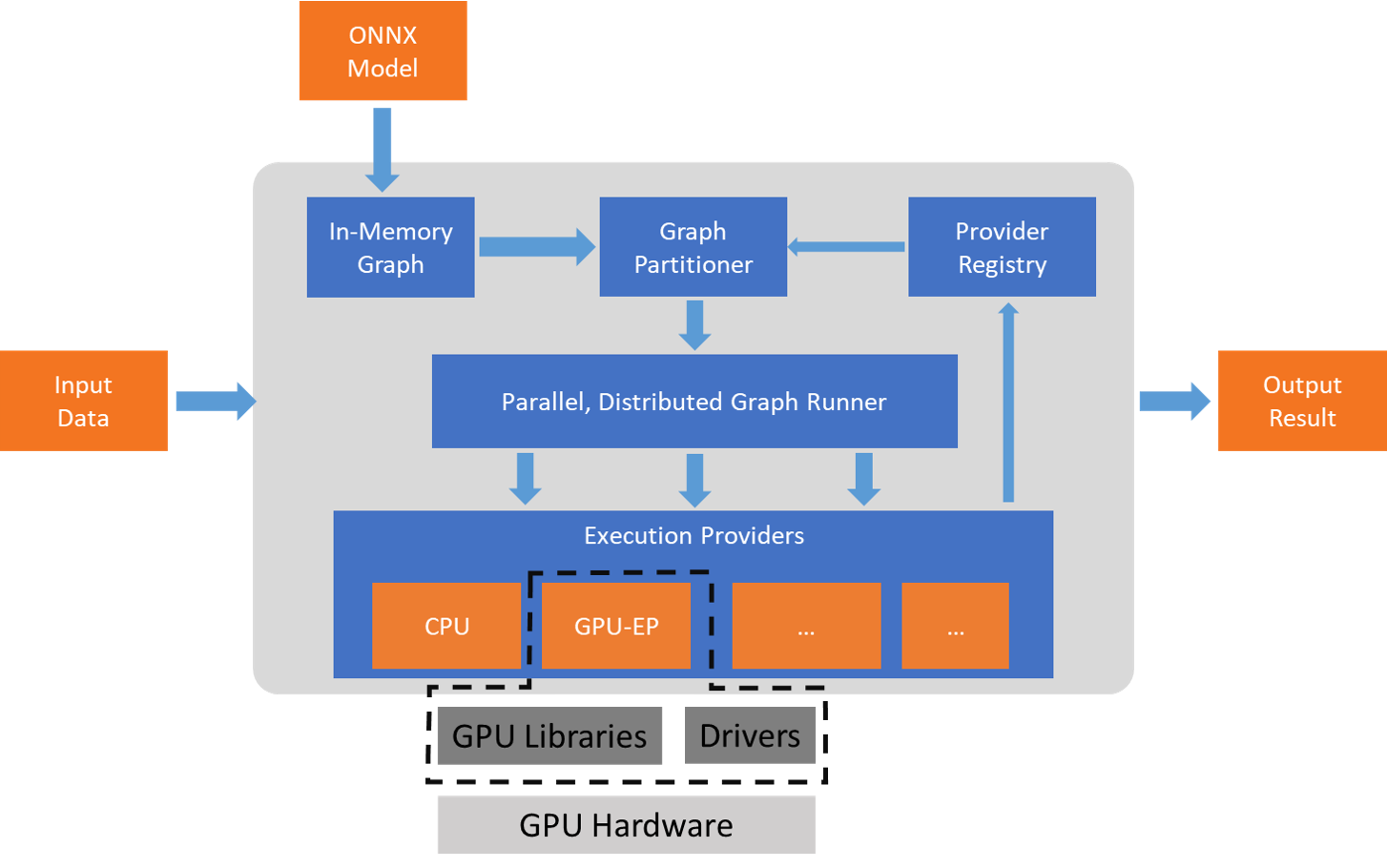
技术栈架构
**1. 系统软件层
- 英伟达:基于CUDA驱动,支持英伟达GPU的底层硬件加速。
- AMD:基于ROCm驱动,支持AMD GPU的底层硬件加速。
**2. 运行时环境层
- 英伟达:ONNX Runtime with CUDA,支持使用CUDA进行硬件加速。
- AMD:ONNX Runtime with ROCm,支持使用ROCm进行硬件加速。
**3. 编程模型和语言层
- 英伟达:通过TensorFlow、PyTorch等框架导出ONNX模型,使用CUDA后端优化编译。
- AMD:通过相同框架导出ONNX模型,但使用ROCm后端优化编译。
**4. 计算库层
- 英伟达:使用cuDNN、TensorRT等计算库来加速ONNX模型的执行。
- AMD:使用MIOpen、rocBLAS等计算库来加速ONNX模型的执行。
**5. 框架层
- ONNX本身在框架层无差异,支持的框架(如PyTorch、TensorFlow)可以跨平台导出和执行ONNX模型。
ONNX(Open Neural Network Exchange)是一个开放的深度学习框架互操作性标准,它允许不同的深度学习框架(如PyTorch、TensorFlow等)之间共享模型。在ONNX的系统软件层中主要包括以下几个方面:
ONNX Runtime ONNX Runtime是ONNX模型的推理引擎,旨在提供高效的模型推理。它支持多种硬件后端,包括CPU和GPU,具体而言,支持NVIDIA GPU和AMD GPU。
- CUDA Execution Provider:针对NVIDIA GPU的优化,利用CUDA来加速模型推理。它支持多种操作和优化,能够充分利用GPU的计算能力。
- ROCm Execution Provider:为AMD GPU提供支持,允许在基于ROCm平台的设备上运行ONNX模型。它能够利用AMD的GPU架构进行高效的推理。
模型优化 ONNX提供了一系列工具来优化模型,使其在GPU上运行更高效。这些优化包括:
- 图优化:通过分析计算图,消除冗余节点和合并操作来减少计算量。
- 量化:将模型从浮点数转换为整数,以减少模型大小和加速推理速度,特别是在GPU上。
硬件加速支持 ONNX支持不同类型的GPU硬件加速,包括:
- NVIDIA Tensor Cores:支持混合精度计算,能够加速深度学习模型的训练和推理。
- AMD ROCm:通过ROCm框架,ONNX能够在AMD GPU上实现高效推理,支持Tensor操作和多线程执行。
集成与兼容性 ONNX Runtime能够与多种深度学习框架集成,确保不同框架之间的模型兼容性,使得开发者可以选择合适的GPU硬件进行部署。
API和开发支持 ONNX提供了一系列API,开发者可以使用这些API来加载模型、配置运行时环境以及管理GPU资源。这些API使得开发者能够方便地在GPU上运行ONNX模型。
运行时环境层
运行时环境层
使用 ONNX Runtime 获取可用的执行提供程序,并通过 rocm-smi 工具输出 AMD GPU 具体信息的 Python 代码示例。
- get_amd_gpu_info():使用 subprocess.run 调用 rocm-smi 工具来获取 AMD GPU 的详细信息。rocm-smi 是 AMD 的工具,用于列出 GPU 的硬件信息。
- check_onnx_runtime_rocm():调用 ONNX Runtime 的 get_available_providers() 方法,列出 ONNX Runtime 中当前可用的执行提供程序。如果 ROCMExecutionProvider 可用,说明 ROCm 执行提供程序可以在 AMD GPU 上运行。
import subprocess
import onnxruntime as ort
# 获取 AMD GPU 信息
def get_amd_gpu_info():
try:
# 使用 rocm-smi 命令获取 GPU 信息
result = subprocess.run(['rocm-smi'], stdout=subprocess.PIPE, stderr=subprocess.PIPE, text=True)
if result.returncode == 0:
print("AMD GPU Info:")
print(result.stdout)
else:
print("Error running rocm-smi:", result.stderr)
except FileNotFoundError:
print("rocm-smi not found. Please install ROCm tools.")
# 检查 ONNX Runtime 是否可以使用 ROCm Execution Provider
def check_onnx_runtime_rocm():
# 获取 ONNX Runtime 中的可用执行提供程序
providers = ort.get_available_providers()
print("Available Execution Providers:", providers)
if 'ROCMExecutionProvider' in providers:
print("ROCM Execution Provider is available!")
else:
print("ROCM Execution Provider is not available.")
if __name__ == "__main__":
# 输出 AMD GPU 信息
get_amd_gpu_info()
# 检查 ONNX Runtime 的可用执行提供程序
check_onnx_runtime_rocm()
结果
AMD GPU Info:
======================================== ROCm System Management Interface ========================================
================================================== Concise Info ==================================================
Device Node IDs Temp Power Partitions SCLK MCLK Fan Perf PwrCap VRAM% GPU%
(DID, GUID) (Edge) (Avg) (Mem, Compute, ID)
==================================================================================================================
0 1 0x73df, 49956 38.0°C 9.0W N/A, N/A, 0 500Mhz 96Mhz 0% auto 203.0W 0% 5%
==================================================================================================================
============================================== End of ROCm SMI Log ===============================================
Available ONNX Runtime Execution Providers:
TensorrtExecutionProvider
CUDAExecutionProvider
CPUExecutionProvider
ROCm Execution Provider is available.
编程模型和语言层
定义了一个自定义的PyTorch操作,并将其导出为ONNX格式。
- 自定义函数:MyAddFunction 继承自 torch.autograd.Function,包含两个主要静态方法:forward(ctx, a, b):调用外部库函数 my_lib.my_add 来计算两个张量 a 和 b 的加法。symbolic(g, a, b):为ONNX定义操作的符号表示,创建一个图节点用于将 a 乘以 2,然后加上 b。
- MyAdd 是 torch.nn.Module 的子类,使用 MyAddFunction。在其 forward 方法中调用 my_add。
- 生成一个形状为 (1, 3, 10, 10) 的随机输入张量。
- 使用 torch.onnx.export 将模型导出为名为 my_add.onnx 的ONNX文件,传入相同的输入张量作为两个参数。
- 加载ONNX模型,并使用相同的输入张量进行推理,输出结果存储在 ort_output 中。
- 通过断言检查PyTorch模型的输出与ONNX模型的输出是否接近,确保导出和操作的正确性。
import torch
import my_lib
class MyAddFunction(torch.autograd.Function):
@staticmethod
def forward(ctx, a, b):
return my_lib.my_add(a, b)
@staticmethod
def symbolic(g, a, b):
two = g.op("Constant", value_t=torch.tensor([2]))
a = g.op('Mul', a, two)
return g.op('Add', a, b)
my_add = MyAddFunction.apply
class MyAdd(torch.nn.Module):
def __init__(self):
super().__init__()
def forward(self, a, b):
return my_add(a, b)
model = MyAdd()
input = torch.rand(1, 3, 10, 10)
torch.onnx.export(model, (input, input), 'my_add.onnx')
torch_output = model(input, input).detach().numpy()
import onnxruntime
import numpy as np
sess = onnxruntime.InferenceSession('my_add.onnx')
ort_output = sess.run(None, {'a': input.numpy(), 'b': input.numpy()})[0]
assert np.allclose(torch_output, ort_output)
演示如何使用 PyTorch 和 ONNX Runtime 在不同设备(如 CPU 或 GPU)上进行推理。具体来说,它通过以下步骤展示了如何使用 ONNX Runtime 来运行一个简单的加法模型(两个张量相加),并使用不同的方式将数据传递到设备上进行计算。
- 模型定义了一个简单的加法运算,它接受两个输入张量 x 和 y,返回它们的加法结果。创建并导出模型为 ONNX 格式,其中 x 和 y 的大小是动态的。
- 根据当前设备是否支持 CUDA(运行在NVIDIA GPU),创建一个 ONNX Runtime 会话,可以在 CPU 或 GPU 上运行模型。
- 在 CPU 上运行模型,输入和输出都是 NumPy 数组。使用 PyTorch 张量运行模型,在设备上使用 PyTorch 张量进行推理。
- 在main函数中,第一个调用 run(),输入 x=[1.0, 2.0, 3.0],y=[4.0, 5.0, 6.0],输出 z=[5.0, 7.0, 9.0]。 第二个调用 run_with_data_on_device(),输入 x=[1.0, 2.0, 3.0, 4.0, 5.0] 和 y=[1.0, 2.0, 3.0, 4.0, 5.0],输出 z=[2.0, 4.0, 6.0, 8.0, 10.0]。 第三个调用 run_with_torch_tensors_on_device(),生成两个随机的 PyTorch 张量,并返回加法结果,如 [0.7023, 1.3127, 1.7289, 0.3982, 0.8386]。 最后一个调用也是 run_with_torch_tensors_on_device(),但这次使用 torch.int64 类型张量,输入 x=ones(5) 和 y=zeros(5),输出 [1, 1, 1, 1, 1]
import numpy as np
import torch
import onnxruntime
MODEL_FILE = '.model.onnx'
DEVICE_NAME = 'cuda' if torch.cuda.is_available() else 'cpu'
DEVICE_INDEX = 0 # Replace this with the index of the device you want to run on
DEVICE=f'{DEVICE_NAME}:{DEVICE_INDEX}'
# A simple model to calculate addition of two tensors
def model():
class Model(torch.nn.Module):
def __init__(self):
super(Model, self).__init__()
def forward(self, x, y):
return x.add(y)
return Model()
# Create an instance of the model and export it to ONNX graph format, with dynamic size for the data
def create_model(type: torch.dtype = torch.float32):
sample_x = torch.ones(3, dtype=type)
sample_y = torch.zeros(3, dtype=type)
torch.onnx.export(model(), (sample_x, sample_y), MODEL_FILE, input_names=["x", "y"], output_names=["z"],
dynamic_axes={"x": {0 : "array_length_x"}, "y": {0: "array_length_y"}})
# Create an ONNX Runtime session with the provided model
def create_session(model: str) -> onnxruntime.InferenceSession:
providers = ['CPUExecutionProvider']
if torch.cuda.is_available():
providers.insert(0, 'CUDAExecutionProvider')
return onnxruntime.InferenceSession(model, providers=providers)
# Run the model on CPU consuming and producing numpy arrays
def run(x: np.array, y: np.array) -> np.array:
session = create_session(MODEL_FILE)
z = session.run(["z"], {"x": x, "y": y})
return z[0]
# Run the model on device consuming and producing ORTValues
def run_with_data_on_device(x: np.array, y: np.array) -> onnxruntime.OrtValue:
session = create_session(MODEL_FILE)
x_ortvalue = onnxruntime.OrtValue.ortvalue_from_numpy(x, DEVICE_NAME, DEVICE_INDEX)
y_ortvalue = onnxruntime.OrtValue.ortvalue_from_numpy(y, DEVICE_NAME, DEVICE_INDEX)
io_binding = session.io_binding()
io_binding.bind_input(name='x', device_type=x_ortvalue.device_name(), device_id=0, element_type=x.dtype, shape=x_ortvalue.shape(), buffer_ptr=x_ortvalue.data_ptr())
io_binding.bind_input(name='y', device_type=y_ortvalue.device_name(), device_id=0, element_type=y.dtype, shape=y_ortvalue.shape(), buffer_ptr=y_ortvalue.data_ptr())
io_binding.bind_output(name='z', device_type=DEVICE_NAME, device_id=DEVICE_INDEX, element_type=x.dtype, shape=x_ortvalue.shape())
session.run_with_iobinding(io_binding)
z = io_binding.get_outputs()
return z[0]
# Run the model on device consuming and producing native PyTorch tensors
def run_with_torch_tensors_on_device(x: torch.Tensor, y: torch.Tensor, np_type: np.dtype = np.float32, torch_type: torch.dtype = torch.float32) -> torch.Tensor:
session = create_session(MODEL_FILE)
binding = session.io_binding()
x_tensor = x.contiguous()
y_tensor = y.contiguous()
binding.bind_input(
name='x',
device_type=DEVICE_NAME,
device_id=DEVICE_INDEX,
element_type=np_type,
shape=tuple(x_tensor.shape),
buffer_ptr=x_tensor.data_ptr(),
)
binding.bind_input(
name='y',
device_type=DEVICE_NAME,
device_id=DEVICE_INDEX,
element_type=np_type,
shape=tuple(y_tensor.shape),
buffer_ptr=y_tensor.data_ptr(),
)
## Allocate the PyTorch tensor for the model output
z_tensor = torch.empty(x_tensor.shape, dtype=torch_type, device=DEVICE).contiguous()
binding.bind_output(
name='z',
device_type=DEVICE_NAME,
device_id=DEVICE_INDEX,
element_type=np_type,
shape=tuple(z_tensor.shape),
buffer_ptr=z_tensor.data_ptr(),
)
session.run_with_iobinding(binding)
return z_tensor
def main():
create_model()
print(run(x=np.float32([1.0, 2.0, 3.0]),y=np.float32([4.0, 5.0, 6.0])))
# [array([5., 7., 9.], dtype=float32)]
print(run_with_data_on_device(x=np.float32([1.0, 2.0, 3.0, 4.0, 5.0]), y=np.float32([1.0, 2.0, 3.0, 4.0, 5.0])).numpy())
# [ 2. 4. 6. 8. 10.]
print(run_with_torch_tensors_on_device(torch.rand(5).to(DEVICE), torch.rand(5).to(DEVICE)))
# tensor([0.7023, 1.3127, 1.7289, 0.3982, 0.8386])
create_model(torch.int64)
print(run_with_torch_tensors_on_device(torch.ones(5, dtype=torch.int64).to(DEVICE), torch.zeros(5, dtype=torch.int64).to(DEVICE), np_type=np.int64, torch_type=torch.int64))
# tensor([1, 1, 1, 1, 1])
if __name__ == "__main__":
main()
可以使用C++和ONNX Runtime来实现类似的加法操作。以下是一个简单的C++示例,它演示了如何使用ONNX Runtime来加载一个简单的加法模型,并运行推理。 使用PyTorch创建一个简单的加法模型并将其导出为ONNX格式:
import torch
class SimpleAddModel(torch.nn.Module):
def forward(self, x, y):
return x + y
# 创建并导出模型
model = SimpleAddModel()
x = torch.randn(3, dtype=torch.float32)
y = torch.randn(3, dtype=torch.float32)
torch.onnx.export(model, (x, y), "simple_add.onnx", input_names=['x', 'y'], output_names=['z'])
- 这段代码将创建一个简单的模型,将两个输入张量 x 和 y 相加,并导出为 simple_add.onnx。 编写C++代码,使用ONNX Runtime加载和运行该模型。
#include <onnxruntime/core/session/onnxruntime_cxx_api.h>
#include <iostream>
#include <vector>
#include <assert.h>
int main() {
// Initialize ONNX Runtime environment
Ort::Env env(ORT_LOGGING_LEVEL_WARNING, "SimpleAdd");
// Create ONNX Runtime session options
Ort::SessionOptions session_options;
session_options.SetIntraOpNumThreads(1);
// Use GPU (CUDA) if available, otherwise fallback to CPU
const char* cuda_provider = "CUDAExecutionProvider";
if (Ort::GetAvailableProviders().count(cuda_provider)) {
session_options.AppendExecutionProvider_CUDA(0); // Device ID 0 for the first GPU
} else {
std::cout << "CUDA provider not available, running on CPU." << std::endl;
}
// Load the ONNX model
const char* model_path = "simple_add.onnx";
Ort::Session session(env, model_path, session_options);
// Get model input/output details
Ort::AllocatorWithDefaultOptions allocator;
// Get the name and shape of the first input tensor ('x')
char* input_name_x = session.GetInputName(0, allocator);
Ort::TypeInfo input_type_info_x = session.GetInputTypeInfo(0);
auto input_tensor_info_x = input_type_info_x.GetTensorTypeAndShapeInfo();
std::vector<int64_t> input_shape_x = input_tensor_info_x.GetShape();
// Get the name and shape of the second input tensor ('y')
char* input_name_y = session.GetInputName(1, allocator);
Ort::TypeInfo input_type_info_y = session.GetInputTypeInfo(1);
auto input_tensor_info_y = input_type_info_y.GetTensorTypeAndShapeInfo();
std::vector<int64_t> input_shape_y = input_tensor_info_y.GetShape();
// Create input data (example: 3-element float vectors)
std::vector<float> input_data_x = {1.0f, 2.0f, 3.0f};
std::vector<float> input_data_y = {4.0f, 5.0f, 6.0f};
// Create input tensor objects for 'x' and 'y'
auto memory_info = Ort::MemoryInfo::CreateCpu(OrtArenaAllocator, OrtMemTypeDefault);
Ort::Value input_tensor_x = Ort::Value::CreateTensor<float>(memory_info, input_data_x.data(), input_data_x.size(), input_shape_x.data(), input_shape_x.size());
Ort::Value input_tensor_y = Ort::Value::CreateTensor<float>(memory_info, input_data_y.data(), input_data_y.size(), input_shape_y.data(), input_shape_y.size());
// Prepare input and output names
const char* input_names[] = {input_name_x, input_name_y};
const char* output_names[] = {"z"};
// Run inference
auto output_tensors = session.Run(Ort::RunOptions{nullptr}, input_names, &input_tensor_x, 2, output_names, 1);
// Get output tensor and data
float* output_data = output_tensors[0].GetTensorMutableData<float>();
// Print the output results
std::cout << "Output (z): ";
for (size_t i = 0; i < input_data_x.size(); i++) {
std::cout << output_data[i] << " ";
}
std::cout << std::endl;
// Clean up
allocator.Free(input_name_x);
allocator.Free(input_name_y);
return 0;
}
- 环境初始化:首先使用 Ort::Env 初始化 ONNX Runtime 环境,并指定日志级别为 ORT_LOGGING_LEVEL_WARNING。
- 加载模型:使用 Ort::Session 加载导出的 simple_add.onnx 模型。
- 输入/输出信息:通过调用 GetInputName() 和 GetInputTypeInfo() 获- 取输入和输出的名称和形状。这里假设输入 x 和 y 的形状为 [3],即长度为3的一维张量。
- 创建输入张量:使用 Ort::Value::CreateTensor 创建包含输入数据的张量,这里是长度为3的浮点数数组。
- 运行推理:通过 session.Run() 执行模型推理,并获取输出张量。
- 输出结果:输出结果将存储在 output_data 中,最后我们将其打印到控制台。 结果
Output (z): 5 7 9
计算库层
ONNX Runtime 以 ONNX 图形格式或 ORT 格式(适用于内存和磁盘有限的环境)加载并执行模型推理。可以根据具体场景选择合适的方式来指定和访问模型所消耗和生成的数据。 InferenceSession 是 ONNX Runtime 的主类。它用于加载和运行 ONNX 模型,以及指定环境和应用程序配置选项。 ONNX Runtime 的推理会话通过 OrtValue 类处理数据的消耗和生成。在 CPU 上(默认),OrtValues 可以映射到本机 Python 数据结构,如 numpy 数组、字典和 numpy 数组列表。通常情况下,ONNX Runtime 会将输入和输出默认放置在 CPU 上。如果输入或输出是在其他设备上进行处理的,将数据放在 CPU 上可能并不是最佳选择,因为这会导致 CPU 与设备之间的数据复制。
# X is numpy array on cpu
ortvalue = onnxruntime.OrtValue.ortvalue_from_numpy(X)
ortvalue.device_name() # 'cpu'
ortvalue.shape() # shape of the numpy array X
ortvalue.data_type() # 'tensor(float)'
ortvalue.is_tensor() # 'True'
np.array_equal(ortvalue.numpy(), X) # 'True'
# ortvalue can be provided as part of the input feed to a model
session = onnxruntime.InferenceSession(
'model.onnx',
providers=['CUDAExecutionProvider', 'CPUExecutionProvider'])
)
results = session.run(["Y"], {"X": ortvalue})
ONNX Runtime 支持自定义数据结构,兼容所有 ONNX 数据格式,允许用户将支持这些格式的数据放置在设备上,例如支持 CUDA 的设备。这一功能称为 IOBinding。
要使用 IOBinding 功能,只需将 InferenceSession.run() 替换为 InferenceSession.run_with_iobinding()。这样,图形可以在 CPU 以外的设备上执行,例如 CUDA,用户可以通过 IOBinding 将数据复制到 GPU 上。
# X is numpy array on cpu
session = onnxruntime.InferenceSession(
'model.onnx',
providers=['CUDAExecutionProvider', 'CPUExecutionProvider'])
)
io_binding = session.io_binding()
# OnnxRuntime will copy the data over to the CUDA device if 'input' is consumed by nodes on the CUDA device
io_binding.bind_cpu_input('input', X)
io_binding.bind_output('output')
session.run_with_iobinding(io_binding)
Y = io_binding.copy_outputs_to_cpu()[0]
输入数据存放在设备上,用户可以直接使用这些输入,而输出数据则保留在 CPU 上。
# X is numpy array on cpu
X_ortvalue = onnxruntime.OrtValue.ortvalue_from_numpy(X, 'cuda', 0)
session = onnxruntime.InferenceSession(
'model.onnx',
providers=['CUDAExecutionProvider', 'CPUExecutionProvider'])
)
io_binding = session.io_binding()
io_binding.bind_input(name='input', device_type=X_ortvalue.device_name(), device_id=0, element_type=np.float32, shape=X_ortvalue.shape(), buffer_ptr=X_ortvalue.data_ptr())
io_binding.bind_output('output')
session.run_with_iobinding(io_binding)
Y = io_binding.copy_outputs_to_cpu()[0
输入数据和输出数据都位于同一设备上,用户可以直接使用输入,同时将输出也保留在该设备上。
#X is numpy array on cpu
X_ortvalue = onnxruntime.OrtValue.ortvalue_from_numpy(X, 'cuda', 0)
Y_ortvalue = onnxruntime.OrtValue.ortvalue_from_shape_and_type([3, 2], np.float32, 'cuda', 0) # Change the shape to the actual shape of the output being bound
session = onnxruntime.InferenceSession(
'model.onnx',
providers=['CUDAExecutionProvider', 'CPUExecutionProvider'])
)
io_binding = session.io_binding()
io_binding.bind_input(
name='input',
device_type=X_ortvalue.device_name(),
device_id=0,
element_type=np.float32,
shape=X_ortvalue.shape(),
buffer_ptr=X_ortvalue.data_ptr()
)
io_binding.bind_output(
name='output',
device_type=Y_ortvalue.device_name(),
device_id=0,
element_type=np.float32,
shape=Y_ortvalue.shape(),
buffer_ptr=Y_ortvalue.data_ptr()
)
session.run_with_iobinding(io_binding)
用户可以请求 ONNX Runtime 在设备上分配输出,这对于动态形状的输出尤其有用。用户可以通过 get_outputs() API 访问与分配的输出对应的 OrtValue。因此,用户可以将 ONNX Runtime 为输出分配的内存作为 OrtValue 使用。
#X is numpy array on cpu
X_ortvalue = onnxruntime.OrtValue.ortvalue_from_numpy(X, 'cuda', 0)
session = onnxruntime.InferenceSession(
'model.onnx',
providers=['CUDAExecutionProvider', 'CPUExecutionProvider'])
)
io_binding = session.io_binding()
io_binding.bind_input(
name='input',
device_type=X_ortvalue.device_name(),
device_id=0,
element_type=np.float32,
shape=X_ortvalue.shape(),
buffer_ptr=X_ortvalue.data_ptr()
)
#Request ONNX Runtime to bind and allocate memory on CUDA for 'output'
io_binding.bind_output('output', 'cuda')
session.run_with_iobinding(io_binding)
# The following call returns an OrtValue which has data allocated by ONNX Runtime on CUDA
ort_output = io_binding.get_outputs()[0]
还可以将输入和输出直接绑定到 PyTorch 张量。
# X is a PyTorch tensor on device
session = onnxruntime.InferenceSession('model.onnx', providers=['CUDAExecutionProvider', 'CPUExecutionProvider']))
binding = session.io_binding()
X_tensor = X.contiguous()
binding.bind_input(
name='X',
device_type='cuda',
device_id=0,
element_type=np.float32,
shape=tuple(x_tensor.shape),
buffer_ptr=x_tensor.data_ptr(),
)
## Allocate the PyTorch tensor for the model output
Y_shape = ... # You need to specify the output PyTorch tensor shape
Y_tensor = torch.empty(Y_shape, dtype=torch.float32, device='cuda:0').contiguous()
binding.bind_output(
name='Y',
device_type='cuda',
device_id=0,
element_type=np.float32,
shape=tuple(Y_tensor.shape),
buffer_ptr=Y_tensor.data_ptr(),
)
session.run_with_iobinding(binding)
ONNX 后端(Backend)框架的一个实现,定义了用于处理和执行 ONNX 模型的基本结构和功能。
- DeviceType 类定义了支持的设备类型,使用 NewType 创建了 CPU 和 CUDA 作为设备类型的常量。
- Device 类用于表示设备及其 ID,构造函数解析设备字符串(如 "CUDA:1"),并设置相应的类型和 ID。
- BackendRep 类表示后端准备执行模型后返回的句柄,提供一个 run 方法用于执行模型。
- Backend 类是 ONNX 模型的执行单元,包含多个类方法,负责模型的兼容性检查、准备和执行。is_compatible:检查模型是否与后端兼容。prepare:准备模型以便重复执行,返回一个 BackendRep 实例。run_model:准备模型并运行,返回结果。run_node:运行单个操作(节点),用于快速测试和验证。supports_device:检查后端是否支持特定设备。
from __future__ import annotations
from collections import namedtuple
from typing import Any, NewType, Sequence
import numpy
import onnx.checker
import onnx.onnx_cpp2py_export.checker as c_checker
from onnx import IR_VERSION, ModelProto, NodeProto
class DeviceType:
"""Describes device type."""
_Type = NewType("_Type", int)
CPU: _Type = _Type(0)
CUDA: _Type = _Type(1)
class Device:
"""Describes device type and device id
syntax: device_type:device_id(optional)
example: 'CPU', 'CUDA', 'CUDA:1'
"""
def __init__(self, device: str) -> None:
options = device.split(":")
self.type = getattr(DeviceType, options[0])
self.device_id = 0
if len(options) > 1:
self.device_id = int(options[1])
def namedtupledict(
typename: str, field_names: Sequence[str], *args: Any, **kwargs: Any
) -> type[tuple[Any, ...]]:
field_names_map = {n: i for i, n in enumerate(field_names)}
# Some output names are invalid python identifier, e.g. "0"
kwargs.setdefault("rename", True)
data = namedtuple(typename, field_names, *args, **kwargs) # type: ignore # noqa: PYI024
def getitem(self: Any, key: Any) -> Any:
if isinstance(key, str):
key = field_names_map[key]
return super(type(self), self).__getitem__(key) # type: ignore
data.__getitem__ = getitem # type: ignore[assignment]
return data
class BackendRep:
"""BackendRep is the handle that a Backend returns after preparing to execute
a model repeatedly. Users will then pass inputs to the run function of
BackendRep to retrieve the corresponding results.
"""
def run(self, inputs: Any, **kwargs: Any) -> tuple[Any, ...]: # noqa: ARG002
"""Abstract function."""
return (None,)
class Backend:
"""Backend is the entity that will take an ONNX model with inputs,
perform a computation, and then return the output.
For one-off execution, users can use run_node and run_model to obtain results quickly.
For repeated execution, users should use prepare, in which the Backend
does all of the preparation work for executing the model repeatedly
(e.g., loading initializers), and returns a BackendRep handle.
"""
@classmethod
def is_compatible(
cls, model: ModelProto, device: str = "CPU", **kwargs: Any # noqa: ARG003
) -> bool:
# Return whether the model is compatible with the backend.
return True
@classmethod
def prepare(
cls, model: ModelProto, device: str = "CPU", **kwargs: Any # noqa: ARG003
) -> BackendRep | None:
# TODO Remove Optional from return type
onnx.checker.check_model(model)
return None
@classmethod
def run_model(
cls, model: ModelProto, inputs: Any, device: str = "CPU", **kwargs: Any
) -> tuple[Any, ...]:
backend = cls.prepare(model, device, **kwargs)
assert backend is not None
return backend.run(inputs)
@classmethod
def run_node(
cls,
node: NodeProto,
inputs: Any, # noqa: ARG003
device: str = "CPU", # noqa: ARG003
outputs_info: ( # noqa: ARG003
Sequence[tuple[numpy.dtype, tuple[int, ...]]] | None
) = None,
**kwargs: dict[str, Any],
) -> tuple[Any, ...] | None:
"""Simple run one operator and return the results.
Args:
node: The node proto.
inputs: Inputs to the node.
device: The device to run on.
outputs_info: a list of tuples, which contains the element type and
shape of each output. First element of the tuple is the dtype, and
the second element is the shape. More use case can be found in
https://github.com/onnx/onnx/blob/main/onnx/backend/test/runner/__init__.py
kwargs: Other keyword arguments.
"""
# TODO Remove Optional from return type
if "opset_version" in kwargs:
special_context = c_checker.CheckerContext()
special_context.ir_version = IR_VERSION
special_context.opset_imports = {"": kwargs["opset_version"]} # type: ignore
onnx.checker.check_node(node, special_context)
else:
onnx.checker.check_node(node)
return None
@classmethod
def supports_device(cls, device: str) -> bool: # noqa: ARG003
"""Checks whether the backend is compiled with particular device support.
In particular it's used in the testing suite.
"""
return True
框架模型层
实现了如何将一个简单的PyTorch模型导出为ONNX格式,优化它,并使用ONNX Runtime进行推理,同时支持AMD GPU(通过ROCm)。以下是代码各部分的简要说明:
- 定义了一个简单的线性模型 (
SimpleModel),它包含一个全连接层。 - 将模型导出为ONNX格式,指定输入和输出名称,设置动态轴以支持批次大小,并配置优化选项。
- 加载导出的ONNX模型,并对单个输入和一批输入进行推理。打印模型的输出结果以验证结果。
- 使用
onnxoptimizer对ONNX模型进行优化,并保存优化后的模型。 - 创建了使用
ROCMExecutionProvider的推理会话,从而允许模型在AMD GPU上运行。打印GPU推理的输出结果。
import torch
import torch.nn as nn
# 定义一个简单的神经网络模型
class SimpleModel(nn.Module):
def __init__(self):
super(SimpleModel, self).__init__()
self.fc = nn.Linear(10, 2) # 一个线性层,输入 10 维,输出 2 维
def forward(self, x):
return self.fc(x)
# 实例化模型
model = SimpleModel()
# 定义模型的输入(1个批次,10维输入)
dummy_input = torch.randn(1, 10)
# 导出模型为 onnx 格式
torch.onnx.export(model, # 要导出的模型
dummy_input, # 模型的输入
"simple_model.onnx", # 导出文件名
export_params=True, # 是否导出参数
opset_version=11, # ONNX 操作集版本
do_constant_folding=True, # 是否执行常量折叠优化
input_names=['input'], # 输入张量的名称
output_names=['output'], # 输出张量的名称
dynamic_axes={'input': {0: 'batch_size'}, # 允许动态批次大小
'output': {0: 'batch_size'}})
import onnxruntime as ort
import numpy as np
# 加载 ONNX 模型
ort_session = ort.InferenceSession("simple_model.onnx")
# 创建一个输入数据(假设是从训练集中获取的)
input_data = np.random.randn(1, 10).astype(np.float32)
# 运行推理
outputs = ort_session.run(
None, # 默认输出
{"input": input_data} # 输入字典,键是我们在导出时定义的输入名称
)
# 输出结果
print("ONNX 模型输出:", outputs)
import onnx
import onnxoptimizer
# 加载刚刚导出的 ONNX 模型
model = onnx.load("simple_model.onnx")
# 使用 onnxoptimizer 对模型进行优化
optimized_model = onnxoptimizer.optimize(model)
# 保存优化后的模型
onnx.save(optimized_model, "optimized_simple_model.onnx")
print("模型优化完成!")
import onnxruntime as ort
import numpy as np
# 加载 ONNX 模型
ort_session = ort.InferenceSession("simple_model.onnx")
# 创建批量输入数据(比如10个样本,每个样本是10维输入)
batch_input_data = np.random.randn(10, 10).astype(np.float32)
# 运行批量推理
batch_outputs = ort_session.run(
None, # 默认输出
{"input": batch_input_data} # 输入字典,键是我们定义的输入名称
)
# 输出批量结果
print("ONNX 模型批量推理输出:", batch_outputs)
import onnxruntime as ort
import numpy as np
# 创建一个带有 AMD GPU 支持的推理会话
providers = ['ROCMExecutionProvider'] # 使用 ROCm(AMD GPU)
ort_session = ort.InferenceSession("simple_model.onnx", providers=providers)
# 创建输入数据
input_data = np.random.randn(1, 10).astype(np.float32)
# 运行 AMD GPU 推理
outputs = ort_session.run(
None, # 默认输出
{"input": input_data} # 输入字典,键是我们定义的输入名称
)
print("使用 AMD GPU 推理输出:", outputs)
结果
ONNX 模型输出: [array([[-0.2806534 , -0.34268075]], dtype=float32)]
模型优化完成!
ONNX 模型批量推理输出: [array([[ 0.72778636, -1.348342 ],
[ 0.38623396, -0.01857646],
[ 0.30792585, 0.5733432 ],
[ 0.43119785, -0.8729425 ],
[ 0.38088942, -0.41258603],
[ 1.1837193 , 0.80213755],
[ 0.5879338 , 0.5948198 ],
[-0.5040427 , -1.1044548 ],
[-0.63992363, -1.0058911 ],
[ 0.55836433, -1.181501 ]], dtype=float32)]
实现了一个简单的卷积神经网络(CNN),使用 PyTorch 进行训练,数据集为 CIFAR-10,然后将模型导出为 ONNX 格式,并使用 ONNX Runtime 和 ROCm 执行提供者进行推理。
- 定义了一个 CNNModel 类,其中包含两个卷积层,后面跟有最大池化层和全连接层。输出层有 10 个单元,对应 CIFAR-10 数据集中的 10 个类别。
- 对 CIFAR-10 图像进行了归一化,提高模型性能。模型训练了 2 个 epoch。
- 加载 ONNX 模型并使用 ROCm 执行提供者进行执行,适合 AMD GPU。
import torch
import torch.nn as nn
import torch.optim as optim
import torchvision
import torchvision.transforms as transforms
import torch.nn.functional as F
# 定义卷积神经网络模型
class CNNModel(nn.Module):
def __init__(self):
super(CNNModel, self).__init__()
self.conv1 = nn.Conv2d(3, 16, 3, padding=1) # 输入为3通道(RGB),输出为16通道
self.pool = nn.MaxPool2d(2, 2)
self.conv2 = nn.Conv2d(16, 32, 3, padding=1)
self.fc1 = nn.Linear(32 * 8 * 8, 120) # CIFAR-10 的图片为32x32
self.fc2 = nn.Linear(120, 84)
self.fc3 = nn.Linear(84, 10) # 10个类别
def forward(self, x):
x = self.pool(F.relu(self.conv1(x)))
x = self.pool(F.relu(self.conv2(x)))
x = x.view(-1, 32 * 8 * 8) # 展平
x = F.relu(self.fc1(x))
x = F.relu(self.fc2(x))
x = self.fc3(x)
return x
# 数据预处理
transform = transforms.Compose([
transforms.ToTensor(),
transforms.Normalize((0.5, 0.5, 0.5), (0.5, 0.5, 0.5)),
])
# 加载 CIFAR-10 数据集
trainset = torchvision.datasets.CIFAR10(root='./data', train=True, download=True, transform=transform)
trainloader = torch.utils.data.DataLoader(trainset, batch_size=4, shuffle=True)
# 创建模型实例
model = CNNModel()
criterion = nn.CrossEntropyLoss()
optimizer = optim.SGD(model.parameters(), lr=0.001, momentum=0.9)
# 训练模型
for epoch in range(2): # 训练2个epoch
for inputs, labels in trainloader:
optimizer.zero_grad()
outputs = model(inputs)
loss = criterion(outputs, labels)
loss.backward()
optimizer.step()
print("模型训练完成!")
# 导出模型为 ONNX 格式
dummy_input = torch.randn(1, 3, 32, 32) # 创建一个虚拟输入(1个样本,3通道,32x32)
onnx_file_path = "cnn_model.onnx"
torch.onnx.export(model, dummy_input, onnx_file_path, export_params=True, opset_version=11)
print(f"模型已导出为 {onnx_file_path}!")
import onnx
import onnxruntime as ort
import numpy as np
# 加载 ONNX 模型
onnx_model = onnx.load(onnx_file_path)
onnx.checker.check_model(onnx_model) # 检查模型的有效性
# 创建 ONNX Runtime 会话,指定使用 AMD
providers = ['ROCmExecutionProvider'] # 指定使用 ROCm 提供程序
session = ort.InferenceSession(onnx_file_path, providers=providers)
# 准备输入数据
input_data = np.random.randn(1, 3, 32, 32).astype(np.float32) # 1个样本,3通道,32x32
# 进行推理
outputs = session.run(None, {session.get_inputs()[0].name: input_data})
print("推理输出:", outputs)
结果
Files already downloaded and verified
模型训练完成!
模型已导出为 cnn_model.onnx!
推理输出: [array([[-0.08859831, 4.2947183 , -0.94107497, -0.48823586, -1.97818 ,
0.16228256, 2.5196002 , -3.419997 , -1.7335896 , 3.3261833 ]],
dtype=float32)]
实现了如何使用PyTorch框架、ONNX框架以及AMD GPU来实现矩阵乘法。这个示例定义了一个简单的模型进行矩阵乘法运算,然后将模型导出为ONNX格式,并使用ONNX Runtime在AMD GPU上进行推理。
import torch
import torch.nn as nn
import onnx
import onnxoptimizer
import onnxruntime as ort
import numpy as np
# 定义一个简单的神经网络模型,用于矩阵乘法
class MatrixMultiplicationModel(nn.Module):
def __init__(self):
super(MatrixMultiplicationModel, self).__init__()
def forward(self, A, B):
return torch.matmul(A, B) # 矩阵乘法
# 实例化模型
model = MatrixMultiplicationModel()
# 创建输入数据(2x3 矩阵和 3x2 矩阵)
A = torch.randn(2, 3, dtype=torch.float32) # 输入矩阵 A
B = torch.randn(3, 2, dtype=torch.float32) # 输入矩阵 B
# 导出模型为ONNX格式
onnx_filename = "matrix_multiplication_model.onnx"
torch.onnx.export(model,
(A, B), # 模型的输入
onnx_filename, # 导出文件名
export_params=True, # 是否导出参数
opset_version=11, # ONNX操作集版本
do_constant_folding=True, # 是否执行常量折叠优化
input_names=['A', 'B'], # 输入张量的名称
output_names=['output'], # 输出张量的名称
dynamic_axes={'A': {0: 'batch_size_A', 1: 'cols_A'}, # 允许动态大小
'B': {0: 'cols_B', 1: 'batch_size_B'},
'output': {0: 'batch_size_A', 1: 'cols_B'}})
print(f"模型已成功导出为 {onnx_filename}")
# 加载刚刚导出的ONNX模型
model = onnx.load(onnx_filename)
# 使用onnxoptimizer对模型进行优化
optimized_model = onnxoptimizer.optimize(model)
# 保存优化后的模型
optimized_filename = "optimized_matrix_multiplication_model.onnx"
onnx.save(optimized_model, optimized_filename)
print(f"优化后的模型已保存为 {optimized_filename}")
# 创建一个支持AMD GPU的推理会话
providers = ['ROCMExecutionProvider'] # 使用ROCm(AMD GPU)
ort_session = ort.InferenceSession(optimized_filename, providers=providers)
# 创建输入数据
A_input = np.random.randn(2, 3).astype(np.float32) # 输入矩阵 A
B_input = np.random.randn(3, 2).astype(np.float32) # 输入矩阵 B
# 运行AMD GPU推理
outputs = ort_session.run(
None, # 默认输出
{"A": A_input, "B": B_input} # 输入字典,键是我们定义的输入名称
)
# 输出结果
print("使用AMD GPU推理输出:", outputs)
结果
模型已成功导出为 matrix_multiplication_model.onnx
优化后的模型已保存为 optimized_matrix_multiplication_model.onn
使用AMD GPU推理输出: [array([[0.05410983, 2.5270827 ],
[0.3073317 , 2.2992258 ]], dtype=float32)]
实现了使用 TensorFlow 创建一个简单的模型,然后将其导出为 ONNX 格式,并使用 AMD GPU 通过 ONNX Runtime 进行推理。
- Sequential: 创建一个顺序模型,层按顺序堆叠。
- Dense: 全连接层。第一层:有 64 个神经元,使用 ReLU 激活函数,输入形状为 (32,),表示每个输入样本有 32 个特征。第二层:有 10 个神经元,使用 Softmax 激活函数,用于多类分类(10 类)。
- optimizer: 使用 Adam 优化器进行训练。loss: 使用稀疏分类交叉熵损失函数,适用于类别标签是整数的情况。metrics: 在训练期间监测模型准确率。
- 将训练好的模型保存为 HDF5 格式的文件 my_model.h5。使用 tf2onnx 将 TensorFlow Keras 模型转换为 ONNX 格式,创建 ONNX Runtime 会话,指定使用 CUDAExecutionProvider,以支持在 GPU 上运行推理。
- run: 进行推理。None 表示返回所有输出,{'dense_input': input_data} 是一个字典,将输入数据传递给模型。
import tensorflow as tf
# 创建一个简单的模型
model = tf.keras.Sequential([
tf.keras.layers.Dense(64, activation='relu', input_shape=(32,)),
tf.keras.layers.Dense(10, activation='softmax')
])
# 编译模型
model.compile(optimizer='adam', loss='sparse_categorical_crossentropy', metrics=['accuracy'])
# 生成一些随机数据进行训练
import numpy as np
x_train = np.random.rand(1000, 32).astype(np.float32)
y_train = np.random.randint(0, 10, size=(1000,)).astype(np.int32)
# 训练模型
model.fit(x_train, y_train, epochs=5)
# 保存模型
model.save('my_model.h5')
import tf2onnx
# 转换模型并保存为 ONNX 格式
model_proto, _ = tf2onnx.convert.from_keras(model, output_path='my_model.onnx')
import onnxruntime as ort
# 创建 ONNX Runtime 会话,指定使用 GPU
providers = ['CUDAExecutionProvider']
session = ort.InferenceSession('my_model.onnx', providers=providers)
# 准备输入数据
input_data = np.random.rand(1, 32).astype(np.float32)
# 进行推理
outputs = session.run(None, {'dense_input': input_data}) # 注意这里的 'dense_input' 需要替换为实际输入层的名称
print(outputs)
结果
[array([[0.1, 0.05, 0.6, 0.15, 0.05, 0.01, 0.01, 0.01, 0.01, 0.01]], dtype=float32)]
Intel 平台
Intel 是一家全球领先的半导体公司,以其强大的中央处理器 (CPU) 和最新推出的图形处理单元 (GPU) 架构在人工智能 (AI) 和高性能计算 (HPC) 领域占据重要地位。Intel 提供从 CPU 到 GPU、AI 专用加速器的一整套硬件解决方案,广泛应用于 AI 训练、推理以及数据中心工作负载。借助其丰富的软件工具生态系统,Intel 平台为开发者提供了强大的硬件加速能力,特别是支持复杂的机器学习和深度学习任务。
除了硬件,Intel 还提供了丰富的软件平台和框架,支持跨架构的异构计算。接下来我们将介绍以下几个重要的 Intel 平台相关技术,并在后续通过 AI 技术栈进行深入分析:
oneAPI
oneAPI 是 Intel 推出的开放标准,旨在为开发者提供一个统一的跨架构编程模型。oneAPI 允许在 CPU、GPU、FPGA 和 AI 加速器上编写高效的并行计算代码,避免开发者在多个硬件平台之间重复编写代码。它包含了一系列工具和库,尤其是适合深度学习和高性能计算的应用开发。
- DPC++ (Data Parallel C++):oneAPI 中的核心编程语言,基于 SYCL 标准,支持跨平台的异构计算。开发者可以通过 DPC++ 编写一次代码,并在多个 Intel 硬件上运行,极大提高了代码的可移植性和开发效率。
oneAPI
技术栈架构
以下是oneAPI在Intel平台上的分层架构,按照系统软件层、运行时环境层、编程模型和语言层、计算库层、框架层进行划分:
1. 系统软件层
- Intel oneAPI 基础软件栈:包括操作系统(Linux、Windows等)和Intel的硬件驱动程序,如Intel GPU驱动、Intel CPU的集成驱动等,oneAPI的硬件层能够支持多种Intel硬件设备,如CPU、GPU、FPGA等。
2. 运行时环境层
- oneAPI Level Zero:这是oneAPI的底层硬件抽象层,用于直接与Intel硬件进行高效交互,提供了与硬件的低级别接口,支持Intel CPU、GPU、FPGA的运行时调度和管理。
- DPC++ Runtime:支持Data Parallel C++(DPC++)程序的运行时环境,DPC++是oneAPI的核心编程语言,运行时负责调度计算任务到适合的硬件设备上。
3. 编程模型和语言层
- DPC++(Data Parallel C++):这是oneAPI的主要编程语言,基于C++,扩展了SYCL标准,允许开发者编写跨架构的并行代码,支持在CPU、GPU和FPGA上运行。
- OpenMP、MPI:除了DPC++,oneAPI还支持传统并行编程模型,如OpenMP用于多线程并行,MPI用于分布式计算。
- 库调用:开发者也可以直接使用oneAPI提供的库,而不是编写底层代码,简化开发。
4. 计算库层
- oneAPI 数学核心库(oneMKL):用于高性能数学计算,支持线性代数、FFT等核心数学操作,在Intel硬件上进行了高度优化。
- oneAPI 数据分析库(oneDAL):提供机器学习和数据分析的高效实现。
- oneAPI 深度神经网络库(oneDNN):用于深度学习推理和训练的高效加速,支持卷积操作、激活函数等基础操作。
- oneAPI Video Processing Library(oneVPL):用于加速视频编码、解码和处理。
5. 框架层
- TensorFlow、PyTorch等集成:通过oneDNN等库,oneAPI可以加速深度学习框架如TensorFlow、PyTorch的执行,优化Intel硬件上神经网络的训练和推理性能。
- HPC框架集成:对于高性能计算(HPC),oneAPI支持与多个科学计算框架的集成,例如通过oneMKL优化数值计算库。
系统软件层
系统软件层是指在硬件和应用程序之间起到连接和管理作用的软件栈。这一层次的软件负责硬件资源的分配、管理和调度,确保应用程序能够有效地利用底层硬件设备。对于Intel的生态系统,系统软件层主要包括操作系统、硬件驱动程序以及Intel的oneAPI基础软件栈。
Intel oneAPI 基础软件栈
Intel oneAPI 是一套用于跨多种Intel硬件设备(如CPU、GPU、FPGA等)的统一编程框架,旨在帮助开发者更高效地开发应用程序。提供对Intel多种硬件(CPU、GPU、FPGA等)的统一支持。其系统软件层主要包括操作系统(如Linux、Windows)以及Intel的硬件驱动程序(CPU、GPU、FPGA驱动等),确保oneAPI能够高效利用硬件资源,帮助开发者加速计算、图形处理和数据分析任务。其基础软件栈可以分为以下几个重要部分:
1. 操作系统层
- 支持的操作系统:Intel oneAPI 支持多种主流操作系统,主要包括:
- Linux:常见的发行版包括Ubuntu、Red Hat、CentOS等。Linux通常用于高性能计算、数据中心和开发环境中,具备广泛的开发者支持。
- Windows:用于开发桌面应用程序或在Windows环境中进行研究和开发工作。
操作系统为oneAPI提供底层支持,负责系统资源(如内存、存储、网络)的管理和调度,同时作为硬件与应用程序之间的接口层。
2. Intel 硬件驱动程序
- Intel GPU驱动程序:oneAPI中,Intel GPU驱动负责与Intel集成或独立GPU(如Iris Xe、Arc系列等)进行通信。它允许oneAPI访问GPU的计算资源,支持图形处理和通用计算任务。
- Intel CPU驱动程序:除了操作系统对CPU的基本支持外,Intel提供特定的驱动程序或优化工具,使得oneAPI能够充分利用Intel CPU的多核、多线程架构,提高计算性能。
- FPGA驱动:针对FPGA设备,Intel提供了专门的驱动程序和API接口,oneAPI可以通过这些驱动程序灵活调度FPGA的资源,进行加速计算。
这些驱动程序是硬件设备与操作系统、开发环境交互的桥梁,确保oneAPI能够无缝访问和控制不同硬件的功能。
3. oneAPI 硬件支持层
oneAPI 的硬件支持层是其核心部分,确保能够支持和兼容多种Intel硬件。主要的硬件设备包括:
- CPU:oneAPI支持包括Intel Xeon、Core等系列的CPU。它可以在单机和集群环境下运行,能够处理复杂的并行任务。
- GPU:支持Intel的集成和独立GPU。oneAPI通过DPC++(Data Parallel C++)编程模型,允许开发者编写跨CPU和GPU并行运行的代码。
- FPGA:Intel的FPGA硬件能够通过oneAPI访问,使得开发者可以利用硬件的可编程特性进行计算任务加速。
运行时环境层
检测Intel GPU是否可用,并在GPU上执行一个简单的矩阵乘法操作,同时打印设备的详细信息和运算结果。
- torch.xpu.get_device_name(device): 获取当前设备的名称。返回的设备名称会显示出来。
- torch.xpu.get_device_properties(device): 获取该设备的详细信息,例如总内存等。
- device_properties.total_memory:设备的总内存(以字节为单位),此处将其转换为GB并输出。
- torch.randn(1000, 1000, device=device): 创建两个1000x1000的随机张量tensor_a和tensor_b,并将它们分配到Intel GPU上(通过device=device指定设备)。这些张量在XPU上进行初始化,意味着所有后续的计算都将在XPU上执行。
- torch.matmul(tensor_a, tensor_b): 进行矩阵乘法运算。此运算也将在Intel GPU上进行。
- result.shape: 打印矩阵乘法结果的形状,这里应该是(1000, 1000)。result.sum().item(): 计算并打印结果张量所有元素的总和。
import torch
import intel_extension_for_pytorch as ipex
# 检查当前是否支持Intel GPU
if torch.xpu.is_available():
device = torch.device("xpu")
print("Intel GPU is available.")
# 获取设备名称
device_name = torch.xpu.get_device_name(device)
print(f"Device Name: {device_name}")
# 打印更多设备信息
device_properties = torch.xpu.get_device_properties(device)
print("Detailed Device Information:")
print(f" - Total Memory: {device_properties.total_memory / (1024 ** 3):.2f} GB")
print("Intel GPU is available. Running on:", torch.xpu.get_device_name(device))
# 创建两个随机张量并移动到 Intel GPU
tensor_a = torch.randn(1000, 1000, device=device)
tensor_b = torch.randn(1000, 1000, device=device)
# 在GPU上进行矩阵乘法
result = torch.matmul(tensor_a, tensor_b)
# 打印结果的一些信息
print(f"Result shape: {result.shape}")
print(f"Sum of elements: {result.sum().item()}")
else:
print("Intel GPU is not available.")
结果
Intel GPU is available.
Device Name: Intel(R) Arc(TM) A770 Graphics
Detailed Device Information:
- Total Memory: 15.11 GB
Intel GPU is available. Running on: Intel(R) Arc(TM) A770 Graphics
Result shape: torch.Size([1000, 1000])
Sum of elements: 24389.48828125
编程模型和语言层
通过在 Intel XPU 上执行矩阵乘法,展示了如何使用 PyTorch 和 Intel 扩展库进行计算,并记录了执行时间和输出结果。
- 使用 torch.rand 创建两个 1000x1000 的随机矩阵 A 和 B,并将它们分配到指定的设备(即 XPU)。
- 使用 time.time() 记录开始时间。执行矩阵乘法 C = torch.mm(A, B),计算矩阵 A 和 B 的乘积,并将结果存储在矩阵 C 中。记录结束时间。
- 输出矩阵乘法的结果 C。输出结果矩阵 C 的第一个元素 C[0, 0].item(),使用 .item() 将张量的标量值提取为 Python 数值。计算并输出执行时间,格式化为小数点后六位。
import torch
import intel_extension_for_pytorch as ipex
import time
# 设置设备为 Intel XPU
device = 'xpu'
print(device)
# 创建两个随机矩阵
A = torch.rand(1000, 1000, device=device)
B = torch.rand(1000, 1000, device=device)
start_time = time.time()
C = torch.mm(A, B) # 矩阵乘法
end_time = time.time()
# 输出结果和执行时间
print("矩阵乘法结果:", C)
print("矩阵乘法结果的第一个元素:", C[0, 0].item())
print("执行时间: {:.6f}秒".format(end_time - start_time))
结果
xpu
矩阵乘法结果: tensor([[246.4091, 255.5069, 252.2399, ..., 247.3566, 251.4520, 261.5430],
[252.0482, 253.8953, 248.0201, ..., 246.2549, 249.1073, 261.2542],
[244.2107, 255.6172, 245.4884, ..., 245.6505, 246.0593, 252.1882],
...,
[242.1431, 245.1475, 241.2979, ..., 246.3311, 243.1896, 253.1462],
[245.9689, 248.1380, 245.4601, ..., 245.5615, 247.0750, 255.7415],
[237.5993, 248.8701, 236.9447, ..., 238.5728, 240.6091, 247.0459]],
device='xpu:0')
矩阵乘法结果的第一个元素: 246.4091339111328
执行时间: 0.072625秒
在 Intel XPU 上实现矩阵加法和减法的示例代码
- 记录加法开始时间。使用 C_add = A + B 计算矩阵加法。记录加法结束时间。
- 记录减法开始时间。使用 C_sub = A - B 计算矩阵减法。记录减法结束时间。
import torch
import intel_extension_for_pytorch as ipex
import time
# 设置设备为 Intel XPU
device = 'xpu'
# 创建两个随机矩阵
A = torch.rand(1000, 1000, device=device)
B = torch.rand(1000, 1000, device=device)
# 矩阵加法
start_time_add = time.time()
C_add = A + B # 矩阵加法
end_time_add = time.time()
# 矩阵减法
start_time_sub = time.time()
C_sub = A - B # 矩阵减法
end_time_sub = time.time()
# 输出结果和执行时间
print("矩阵加法结果的第一个元素:", C_add[0, 0].item())
print("矩阵加法执行时间: {:.6f}秒".format(end_time_add - start_time_add))
print("矩阵减法结果的第一个元素:", C_sub[0, 0].item())
print("矩阵减法执行时间: {:.6f}秒".format(end_time_sub - start_time_sub))
结果
矩阵加法结果的第一个元素: 1.158061146736145
矩阵加法执行时间: 0.004714秒
矩阵减法结果的第一个元素: -0.2508704960346222
矩阵减法执行时间: 0.000067秒
代码展示了如何在 Intel XPU 上优化和运行一个预训练的 ResNet50 模型,适合进行快速推理测试。
- 加载预训练的 ResNet50 模型,并设置为评估模式。创建一个随机输入数据 data,其形状为 (1, 3, 224, 224),对应于一张 224x224 的 RGB 图像。
- 将模型和输入数据移动到 Intel XPU 上。使用 ipex.optimize(model) 优化模型,以提高性能。
- 在不计算梯度的情况下执行模型推理,以节省内存和计算资源。输出执行结束的提示。
import torch
import torchvision.models as models
############# code changes ###############
import intel_extension_for_pytorch as ipex
############# code changes ###############
model = models.resnet50(weights="ResNet50_Weights.DEFAULT")
model.eval()
data = torch.rand(1, 3, 224, 224)
######## code changes #######
model = model.to("xpu")
data = data.to("xpu")
model = ipex.optimize(model)
######## code changes #######
with torch.no_grad():
model(data)
print("Execution finished")
结果
Execution finished
使用英特尔的 PyTorch 扩展(IPEX)对一个预训练的 ResNet-50 模型进行静态量化,并通过校准数据优化模型的性能,最终将量化后的模型保存为文件。这样处理后的模型在推理时会更高效,占用的存储空间也会减少。
- intel_extension_for_pytorch: 提供针对英特尔硬件的 PyTorch 模型优化。prepare 和 convert: 准备模型以进行量化和将模型转换为量化格式的函数。torchvision.models: 包含像 ResNet 这样的预训练模型。torchvision: 包含数据集和数据预处理转换。
- 使用 model.eval() 将模型切换到评估模式,禁用丢弃层和批量归一化层。创建一个形状为 (128, 3, 224, 224) 的随机张量 data,用于示例输入。
- 使用 ipex.quantization.default_static_qconfig_mapping 获取默认的静态量化配置映射。代码中提供了一个示例,展示如何自定义量化配置(注释部分)。
- 调用 prepare 函数为量化准备模型,指定量化配置映射和示例输入。inplace=False 表示不在原地修改模型。
- 使用 torchvision.transforms 进行数据预处理,包括调整大小、转换为张量和归一化。创建数据集并通过 DataLoader 加载,用于后续的模型校准。
- 在无梯度计算的上下文中,遍历数据加载器进行模型校准。对每个批次的数据调用准备好的模型,以进行量化校准。
- 调用 convert 函数将准备好的模型转换为量化模型。使用 torch.jit.trace 跟踪转换后的模型,以便生成一个可优化的 TorchScript 模型。使用 torch.jit.freeze 冻结模型,进一步优化其性能。
import torchvision
DOWNLOAD = True
DATA = "/tmp/datasets/cifar10/"
transform = torchvision.transforms.Compose(
[
torchvision.transforms.Resize((224, 224)),
torchvision.transforms.ToTensor(),
torchvision.transforms.Normalize((0.5, 0.5, 0.5), (0.5, 0.5, 0.5)),
]
)
train_dataset = torchvision.datasets.CIFAR10(
root=DATA,
train=True,
transform=transform,
download=DOWNLOAD,
)
calibration_data_loader = torch.utils.data.DataLoader(
dataset=train_dataset, batch_size=512
)
with torch.no_grad():
for batch_idx, (d, target) in enumerate(calibration_data_loader):
print(f"calibrated on batch {batch_idx} out of {len(calibration_data_loader)}")
prepared_model(d)
############################## # noqa F401
converted_model = convert(prepared_model)
with torch.no_grad():
traced_model = torch.jit.trace(converted_model, data)
traced_model = torch.jit.freeze(traced_model)
traced_model.save("static_quantized_model.pt")
print("Saved model to: static_quantized_model.pt")
结果
calibrated on batch 0 out of 98
calibrated on batch 1 out of 98
calibrated on batch 2 out of 98
...
calibrated on batch 96 out of 98
calibrated on batch 97 out of 98
calibrated on batch 98 out of 98
Saved model to: static_quantized_model.pt
计算库层
使用 DPC++ 和 Intel oneAPI MKL 库进行通用矩阵乘法(GEMM)的示例。
- 引入了必要的头文件,包括 STL、SYCL 和 oneAPI MKL,设置了异常处理器用于捕获和处理异步异常。
- 定义了矩阵 A、B 和 C 的维度,以及标量 alpha 和 beta 的值。使用 set_fp_value 函数设置浮点数值。
- 使用 SYCL 设备( CPU 或 GPU)创建执行队列,并分配矩阵内存。矩阵数据从主机复制到设备内存。
- 调用 oneapi::mkl::blas::column_major::gemm 进行矩阵乘法计算。该函数根据给定的矩阵 A 和 B 以及标量 alpha 和 beta 计算 C。
- 计算完成后,将结果从设备内存复制回主机内存,并输出参数及部分矩阵的值。
- 捕获并输出 SYCL 和其他异常信息。初始化设备、打印设备信息并调用 run_gemm_example 执行 GEMM 操作。
// stl includes
#include <algorithm>
#include <cstdlib>
#include <iostream>
#include <vector>
#if __has_include(<sycl/sycl.hpp>)
#include <sycl/sycl.hpp>
#else
#include <CL/sycl.hpp>
#endif
#include "oneapi/mkl.hpp"
#include "example_helper.hpp"
void run_gemm_example(const sycl::device& dev) {
oneapi::mkl::transpose transA = oneapi::mkl::transpose::trans;
oneapi::mkl::transpose transB = oneapi::mkl::transpose::nontrans;
// matrix data sizes
int m = 45;
int n = 98;
int k = 67;
// leading dimensions of data
int ldA = 103;
int ldB = 105;
int ldC = 106;
int sizea = (transA == oneapi::mkl::transpose::nontrans) ? ldA * k : ldA * m;
int sizeb = (transB == oneapi::mkl::transpose::nontrans) ? ldB * n : ldB * k;
int sizec = ldC * n;
// set scalar fp values
float alpha = set_fp_value(float(2.0), float(-0.5));
float beta = set_fp_value(float(3.0), float(-1.5));
// Catch asynchronous exceptions
auto exception_handler = [](sycl::exception_list exceptions) {
for (std::exception_ptr const& e : exceptions) {
try {
std::rethrow_exception(e);
}
catch (sycl::exception const& e) {
std::cerr << "Caught asynchronous SYCL exception during GEMM:" << std::endl;
std::cerr << "\t" << e.what() << std::endl;
}
}
std::exit(2);
};
// create execution queue
sycl::queue main_queue(dev, exception_handler);
sycl::event gemm_done;
sycl::context cxt = main_queue.get_context();
// allocate matrix on host
std::vector<float> A(sizea);
std::vector<float> B(sizeb);
std::vector<float> C(sizec);
std::fill(A.begin(), A.end(), 0);
std::fill(B.begin(), B.end(), 0);
std::fill(C.begin(), C.end(), 0);
rand_matrix(A, transA, m, k, ldA);
rand_matrix(B, transB, k, n, ldB);
rand_matrix(C, oneapi::mkl::transpose::nontrans, m, n, ldC);
// allocate memory on device
auto dev_A = sycl::malloc_device<float>(sizea * sizeof(float), main_queue);
auto dev_B = sycl::malloc_device<float>(sizeb * sizeof(float), main_queue);
auto dev_C = sycl::malloc_device<float>(sizec * sizeof(float), main_queue);
if (!dev_A || !dev_B || !dev_C) {
throw std::runtime_error("Failed to allocate USM memory.");
}
// copy data from host to device
main_queue.memcpy(dev_A, A.data(), sizea * sizeof(float)).wait();
main_queue.memcpy(dev_B, B.data(), sizeb * sizeof(float)).wait();
main_queue.memcpy(dev_C, C.data(), sizec * sizeof(float)).wait();
// add oneapi::mkl::blas::gemm to execution queue
gemm_done = oneapi::mkl::blas::column_major::gemm(main_queue, transA, transB, m, n, k, alpha,
dev_A, ldA, dev_B, ldB, beta, dev_C, ldC);
// Wait until calculations are done
main_queue.wait_and_throw();
// copy data from device back to host
main_queue.memcpy(C.data(), dev_C, sizec * sizeof(float)).wait_and_throw();
std::cout << "\n\t\tGEMM parameters:" << std::endl;
std::cout << "\t\t\ttransA = "
<< (transA == oneapi::mkl::transpose::nontrans
? "nontrans"
: (transA == oneapi::mkl::transpose::trans ? "trans" : "conjtrans"))
<< ", transB = "
<< (transB == oneapi::mkl::transpose::nontrans
? "nontrans"
: (transB == oneapi::mkl::transpose::trans ? "trans" : "conjtrans"))
<< std::endl;
std::cout << "\t\t\tm = " << m << ", n = " << n << ", k = " << k << std::endl;
std::cout << "\t\t\tlda = " << ldA << ", ldB = " << ldB << ", ldC = " << ldC << std::endl;
std::cout << "\t\t\talpha = " << alpha << ", beta = " << beta << std::endl;
std::cout << "\n\t\tOutputting 2x2 block of A,B,C matrices:" << std::endl;
// output the top 2x2 block of A matrix
print_2x2_matrix_values(A.data(), ldA, "A");
// output the top 2x2 block of B matrix
print_2x2_matrix_values(B.data(), ldB, "B");
// output the top 2x2 block of C matrix
print_2x2_matrix_values(C.data(), ldC, "C");
sycl::free(dev_C, main_queue);
sycl::free(dev_B, main_queue);
sycl::free(dev_A, main_queue);
}
void print_example_banner() {
std::cout << "" << std::endl;
std::cout << "########################################################################"
<< std::endl;
std::cout << "# General Matrix-Matrix Multiplication using Unified Shared Memory Example: "
<< std::endl;
std::cout << "# " << std::endl;
std::cout << "# C = alpha * A * B + beta * C" << std::endl;
std::cout << "# " << std::endl;
std::cout << "# where A, B and C are general dense matrices and alpha, beta are" << std::endl;
std::cout << "# floating point type precision scalars." << std::endl;
std::cout << "# " << std::endl;
std::cout << "# Using apis:" << std::endl;
std::cout << "# gemm" << std::endl;
std::cout << "# " << std::endl;
std::cout << "# Using single precision (float) data type" << std::endl;
std::cout << "# " << std::endl;
std::cout << "# Device will be selected during runtime." << std::endl;
std::cout << "# The environment variable ONEAPI_DEVICE_SELECTOR can be used to specify"
<< std::endl;
std::cout << "# available devices" << std::endl;
std::cout << "# " << std::endl;
std::cout << "########################################################################"
<< std::endl;
std::cout << std::endl;
}
int main(int argc, char** argv) {
print_example_banner();
try {
sycl::device dev = sycl::device();
if (dev.is_gpu()) {
std::cout << "Running BLAS GEMM USM example on GPU device." << std::endl;
std::cout << "Device name is: " << dev.get_info<sycl::info::device::name>()
<< std::endl;
}
else {
std::cout << "Running BLAS GEMM USM example on CPU device." << std::endl;
std::cout << "Device name is: " << dev.get_info<sycl::info::device::name>()
<< std::endl;
}
std::cout << "Running with single precision real data type:" << std::endl;
run_gemm_example(dev);
std::cout << "BLAS GEMM USM example ran OK." << std::endl;
}
catch (sycl::exception const& e) {
std::cerr << "Caught synchronous SYCL exception during GEMM:" << std::endl;
std::cerr << "\t" << e.what() << std::endl;
std::cerr << "\tSYCL error code: " << e.code().value() << std::endl;
return 1;
}
catch (std::exception const& e) {
std::cerr << "Caught std::exception during GEMM:" << std::endl;
std::cerr << "\t" << e.what() << std::endl;
return 1;
}
return 0;
}
一个使用 Intel oneAPI 和 SYCL 的快速傅里叶变换 (DFT) 示例,主要功能包括在支持的设备(GPU 或 CPU)上进行复数的原位前向变换。
- 定义 run_example 函数,接收一个 SYCL 设备参数。N 是傅里叶变换的大小,这里设定为 16。
- 定义异步异常处理函数,用于捕获和处理可能出现的 SYCL 异常。创建一个 SYCL 队列并分配共享内存。这里分配了大小为 N * 2 的浮点数组(用于存储复数数据)。
- 创建一个 DFT 描述符,指定数据精度为单精度(float),数据域为实数,变换大小为 N。
- 调用前向 DFT 计算,传入描述符和输入数据的指针,返回计算事件。等待 DFT 计算完成,确保后续操作在变换完成后进行。
- 调用 print_example_banner() 函数以显示示例信息。
- 判断设备类型(GPU 或 CPU),并输出设备名称。捕获不同类型的异常并输出错误信息,确保程序能够正确处理错误。
// stl includes
#include <iostream>
#include <cstdint>
// oneMKL/SYCL includes
#if __has_include(<sycl/sycl.hpp>)
#include <sycl/sycl.hpp>
#else
#include <CL/sycl.hpp>
#endif
#include "oneapi/mkl.hpp"
void run_example(const sycl::device& dev) {
constexpr std::size_t N = 16;
// Catch asynchronous exceptions
auto exception_handler = [](sycl::exception_list exceptions) {
for (std::exception_ptr const& e : exceptions) {
try {
std::rethrow_exception(e);
}
catch (sycl::exception const& e) {
std::cerr << "Caught asynchronous SYCL exception:" << std::endl;
std::cerr << "\t" << e.what() << std::endl;
}
}
std::exit(2);
};
std::cout << "DFT example run_time dispatch" << std::endl;
sycl::queue sycl_queue(dev, exception_handler);
auto x_usm = sycl::malloc_shared<float>(N * 2, sycl_queue);
// 1. create descriptors
oneapi::mkl::dft::descriptor<oneapi::mkl::dft::precision::SINGLE,
oneapi::mkl::dft::domain::REAL>
desc(static_cast<std::int64_t>(N));
// 2. variadic set_value
desc.set_value(oneapi::mkl::dft::config_param::NUMBER_OF_TRANSFORMS,
static_cast<std::int64_t>(1));
desc.set_value(oneapi::mkl::dft::config_param::PLACEMENT,
oneapi::mkl::dft::config_value::INPLACE);
// 3. commit_descriptor (runtime dispatch)
desc.commit(sycl_queue);
// 4. compute_forward / compute_backward (runtime dispatch)
auto compute_event = oneapi::mkl::dft::compute_forward(desc, x_usm);
// Do something with transformed data.
compute_event.wait();
// 5. Free USM allocation.
sycl::free(x_usm, sycl_queue);
}
void print_example_banner() {
std::cout << "########################################################################\n"
"# DFT complex in-place forward transform with USM API example:\n"
"#\n"
"# Using APIs:\n"
"# USM forward complex in-place\n"
"# Run-time dispatch\n"
"#\n"
"# Using single precision (float) data type\n"
"#\n"
"# Device will be selected during runtime.\n"
"# The environment variable ONEAPI_DEVICE_SELECTOR can be used to specify\n"
"# available devices\n"
"#\n"
"########################################################################\n"
<< std::endl;
}
int main(int /*argc*/, char** /*argv*/) {
print_example_banner();
try {
sycl::device my_dev((sycl::default_selector_v));
if (my_dev.is_gpu()) {
std::cout << "Running DFT complex forward example on GPU device" << std::endl;
std::cout << "Device name is: " << my_dev.get_info<sycl::info::device::name>()
<< std::endl;
}
else {
std::cout << "Running DFT complex forward example on CPU device" << std::endl;
std::cout << "Device name is: " << my_dev.get_info<sycl::info::device::name>()
<< std::endl;
}
std::cout << "Running with single precision real data type:" << std::endl;
run_example(my_dev);
std::cout << "DFT example ran OK" << std::endl;
}
catch (oneapi::mkl::unimplemented const& e) {
std::cerr << "Unsupported Configuration:" << std::endl;
std::cerr << "\t" << e.what() << std::endl;
return 0;
}
catch (sycl::exception const& e) {
std::cerr << "Caught synchronous SYCL exception:" << std::endl;
std::cerr << "\t" << e.what() << std::endl;
std::cerr << "\tSYCL error code: " << e.code().value() << std::endl;
return 1;
}
catch (std::exception const& e) {
std::cerr << "Caught std::exception:" << std::endl;
std::cerr << "\t" << e.what() << std::endl;
return 1;
}
return 0;
}
使用 Intel oneAPI MKL 在 SYCL 设备上进行 LU 分解和求解线性方程组
- 定义 run_getrs_example 函数,接收一个 SYCL 设备参数。
- 定义矩阵的尺寸和主维度。m、n 是矩阵 A 的行和列,nrhs 是右侧矩阵 B 的列数。
- 在主机上初始化矩阵 A 和 B,并填充为零。用随机数据填充矩阵 A 和 B。为矩阵 A、B 和 IPIV(pivot index)分配设备内存。获取 LU 分解和求解所需的 scratchpad 大小。将主机上的数据复制到设备。
- 在设备上执行 LU 分解和求解操作。将结果从设备复制回主机,并打印矩阵 A 和解矩阵 X 的前 2x2 块。释放在设备上分配的所有内存。
- 调用 print_example_banner(),选择设备并执行 LU 分解示例。检查所选设备是 CPU 还是 GPU,并输出设备名称。
// STL includes
#include <algorithm>
#include <cstdlib>
#include <iostream>
#include <vector>
// oneMKL/SYCL includes
#if __has_include(<sycl/sycl.hpp>)
#include <sycl/sycl.hpp>
#else
#include <CL/sycl.hpp>
#endif
#include "oneapi/mkl.hpp"
// local includes
#include "example_helper.hpp"
void run_getrs_example(const sycl::device& device) {
// Matrix sizes and leading dimensions
std::int64_t m = 23;
std::int64_t n = 23;
std::int64_t nrhs = 23;
std::int64_t lda = 32;
std::int64_t ldb = 32;
std::int64_t A_size = n * lda;
std::int64_t B_size = nrhs * ldb;
std::int64_t ipiv_size = n;
oneapi::mkl::transpose trans = oneapi::mkl::transpose::nontrans;
// Asynchronous error handler
auto error_handler = [&](sycl::exception_list exceptions) {
for (auto const& e : exceptions) {
try {
std::rethrow_exception(e);
}
catch (oneapi::mkl::lapack::exception const& e) {
// Handle LAPACK related exceptions that happened during asynchronous call
std::cerr << "Caught asynchronous LAPACK exception during GETRF or GETRS:"
<< std::endl;
std::cerr << "\t" << e.what() << std::endl;
std::cerr << "\tinfo: " << e.info() << std::endl;
}
catch (sycl::exception const& e) {
// Handle not LAPACK related exceptions that happened during asynchronous call
std::cerr << "Caught asynchronous SYCL exception during GETRF or GETRS:"
<< std::endl;
std::cerr << "\t" << e.what() << std::endl;
}
}
std::exit(2);
};
// Data preparation on host
std::vector<float> A(A_size);
std::vector<float> B(B_size);
std::fill(A.begin(), A.end(), 0);
std::fill(B.begin(), B.end(), 0);
rand_matrix(A, trans, m, n, lda);
rand_matrix(B, trans, n, nrhs, ldb);
// Data preparation on selected device
sycl::queue queue(device, error_handler);
sycl::context context = queue.get_context();
sycl::event getrf_done;
sycl::event getrs_done;
float* dev_A = sycl::malloc_device<float>(A_size * sizeof(float), queue);
float* dev_B = sycl::malloc_device<float>(B_size * sizeof(float), queue);
std::int64_t* dev_ipiv =
sycl::malloc_device<std::int64_t>(ipiv_size * sizeof(std::int64_t), queue);
std::int64_t getrf_scratchpad_size =
oneapi::mkl::lapack::getrf_scratchpad_size<float>(queue, m, n, lda);
std::int64_t getrs_scratchpad_size =
oneapi::mkl::lapack::getrs_scratchpad_size<float>(queue, trans, n, nrhs, lda, ldb);
float* getrf_scratchpad =
sycl::malloc_shared<float>(getrf_scratchpad_size * sizeof(float), device, context);
float* getrs_scratchpad =
sycl::malloc_shared<float>(getrs_scratchpad_size * sizeof(float), device, context);
if (!dev_A || !dev_B || !dev_ipiv) {
throw std::runtime_error("Failed to allocate USM memory.");
}
// Skip checking getrf scratchpad memory allocation on rocsolver because with rocsolver
// backend getrf does not use scrachpad memory
if (device.is_cpu() || device.get_info<sycl::info::device::vendor_id>() != AMD_ID) {
if (!getrf_scratchpad) {
throw std::runtime_error("Failed to allocate USM memory.");
}
}
// Skip checking getrs scratchpad memory allocation on cusolver/rocsolver because with
// cusolver/rocsolver backend getrs does not use scrachpad memory
if (device.is_cpu() || (device.get_info<sycl::info::device::vendor_id>() != NVIDIA_ID &&
device.get_info<sycl::info::device::vendor_id>() != AMD_ID)) {
if (!getrs_scratchpad) {
throw std::runtime_error("Failed to allocate USM memory.");
}
}
// copy data from host to device
queue.memcpy(dev_A, A.data(), A_size * sizeof(float)).wait();
queue.memcpy(dev_B, B.data(), B_size * sizeof(float)).wait();
// Execute on device
getrf_done = oneapi::mkl::lapack::getrf(queue, m, n, dev_A, lda, dev_ipiv, getrf_scratchpad,
getrf_scratchpad_size);
getrs_done =
oneapi::mkl::lapack::getrs(queue, trans, n, nrhs, dev_A, lda, dev_ipiv, dev_B, ldb,
getrs_scratchpad, getrs_scratchpad_size, { getrf_done });
// Wait until calculations are done
queue.wait_and_throw();
// Copy data from device back to host
queue.memcpy(B.data(), dev_B, B_size * sizeof(float)).wait_and_throw();
// Print results
std::cout << "\n\t\tGETRF and GETRS parameters:" << std::endl;
std::cout << "\t\t\ttrans = "
<< (trans == oneapi::mkl::transpose::nontrans
? "nontrans"
: (trans == oneapi::mkl::transpose::trans ? "trans" : "conjtrans"))
<< std::endl;
std::cout << "\t\t\tm = " << m << ", n = " << n << ", nrhs = " << nrhs << std::endl;
std::cout << "\t\t\tlda = " << lda << ", ldb = " << ldb << std::endl;
std::cout << "\n\t\tOutputting 2x2 block of A and X matrices:" << std::endl;
// output the top 2x2 block of A matrix
print_2x2_matrix_values(A.data(), lda, "A");
// output the top 2x2 block of X matrix
print_2x2_matrix_values(B.data(), ldb, "X");
sycl::free(getrs_scratchpad, queue);
sycl::free(getrf_scratchpad, queue);
sycl::free(dev_ipiv, queue);
sycl::free(dev_B, queue);
sycl::free(dev_A, queue);
}
void print_example_banner() {
std::cout << "" << std::endl;
std::cout << "########################################################################"
<< std::endl;
std::cout << "# LU Factorization and Solve Example: " << std::endl;
std::cout << "# " << std::endl;
std::cout << "# Computes LU Factorization A = P * L * U" << std::endl;
std::cout << "# and uses it to solve for X in a system of linear equations:" << std::endl;
std::cout << "# AX = B" << std::endl;
std::cout << "# where A is a general dense matrix and B is a matrix whose columns" << std::endl;
std::cout << "# are the right-hand sides for the systems of equations." << std::endl;
std::cout << "# " << std::endl;
std::cout << "# Using apis:" << std::endl;
std::cout << "# getrf and getrs" << std::endl;
std::cout << "# " << std::endl;
std::cout << "# Using single precision (float) data type" << std::endl;
std::cout << "# " << std::endl;
std::cout << "# Device will be selected during runtime." << std::endl;
std::cout << "# The environment variable ONEAPI_DEVICE_SELECTOR can be used to specify"
<< std::endl;
std::cout << "# available devices" << std::endl;
std::cout << "# " << std::endl;
std::cout << "########################################################################"
<< std::endl;
std::cout << std::endl;
}
int main(int argc, char** argv) {
print_example_banner();
try {
sycl::device dev = sycl::device();
if (dev.is_gpu()) {
std::cout << "Running LAPACK getrs example on GPU device." << std::endl;
std::cout << "Device name is: " << dev.get_info<sycl::info::device::name>()
<< std::endl;
}
else {
std::cout << "Running LAPACK getrs example on CPU device." << std::endl;
std::cout << "Device name is: " << dev.get_info<sycl::info::device::name>()
<< std::endl;
}
std::cout << "Running with single precision real data type:" << std::endl;
run_getrs_example(dev);
std::cout << "LAPACK GETRS USM example ran OK" << std::endl;
}
catch (oneapi::mkl::lapack::exception const& e) {
// Handle LAPACK related exceptions that happened during synchronous call
std::cerr << "Caught synchronous LAPACK exception:" << std::endl;
std::cerr << "\t" << e.what() << std::endl;
std::cerr << "\tinfo: " << e.info() << std::endl;
return 1;
}
catch (sycl::exception const& e) {
// Handle not LAPACK related exceptions that happened during synchronous call
std::cerr << "Caught synchronous SYCL exception:" << std::endl;
std::cerr << "\t" << e.what() << std::endl;
std::cerr << "\tSYCL error code: " << e.code().value() << std::endl;
return 1;
}
catch (std::exception const& e) {
// Handle not SYCL related exceptions that happened during synchronous call
std::cerr << "Caught synchronous std::exception:" << std::endl;
std::cerr << "\t" << e.what() << std::endl;
return 1;
}
return 0;
}
使用DPC++ (Data Parallel C++) 和 oneAPI 数学核心库(oneMKL)生成均匀分布随机数的示例。使用SYCL (Standard C++ for Heterogeneous Computing) 编程模型,能够在不同硬件设备(如CPU、GPU)上生成随机数,具体使用了Philox4x32x10随机数生成器和Unified Shared Memory (USM) API来进行内存管理。
- seed:随机数生成器的种子值,确保生成相同的随机序列。n:要生成的随机数的数量,这里为1000个。a 和 b:随机数的范围,从0.0到10.0。定义了一个异步异常处理器,当在SYCL的队列执行过程中发生异常时,能够捕捉并处理这些异常。
- sycl::queue queue(dev, exception_handler); 创建了一个SYCL队列,该队列会根据传入的设备对象(dev)选择执行平台(如CPU或GPU),并在出现异常时调用exception_handler。
- oneapi::mkl::rng::default_engine engine(queue, seed); 使用默认的RNG引擎,并根据给定的种子进行初始化。oneapi::mkl::rng::uniform
distribution(a, b); 使用均匀分布生成器,生成范围在a到b之间的浮点数。 - 使用sycl::malloc_device为设备端分配USM内存,用来存放随机数。oneapi::mkl::rng::generate生成随机数并将其存放在设备端的USM内存中。随后将生成的随机数从设备端内存复制回主机端进行处理。
- 生成完毕后,代码将前10个随机数输出到控制台。调用run_uniform_example来生成随机数并处理异常。如果运行成功,则输出随机数生成正常结束的信息。
// stl includes
#include <algorithm>
#include <cstdlib>
#include <iostream>
#include <vector>
// oneMKL/SYCL includes
#if __has_include(<sycl/sycl.hpp>)
#include <sycl/sycl.hpp>
#else
#include <CL/sycl.hpp>
#endif
#include "oneapi/mkl.hpp"
// local includes
#include "example_helper.hpp"
void run_uniform_example(const sycl::device& dev) {
constexpr std::uint64_t seed = 777;
constexpr std::size_t n = 1000;
constexpr std::size_t n_print = 10;
constexpr std::size_t alignment = 64;
// Catch asynchronous exceptions
auto exception_handler = [](sycl::exception_list exceptions) {
for (std::exception_ptr const& e : exceptions) {
try {
std::rethrow_exception(e);
}
catch (sycl::exception const& e) {
std::cerr << "Caught asynchronous SYCL exception during generation:" << std::endl;
std::cerr << "\t" << e.what() << std::endl;
}
}
std::exit(2);
};
sycl::queue queue(dev, exception_handler);
// set scalar Type values
float a(0.0);
float b(10.0);
oneapi::mkl::rng::default_engine engine(queue, seed);
oneapi::mkl::rng::uniform<float> distribution(a, b);
std::vector<float> r(n);
// Data preparation on selected device
float* dev_r = sycl::malloc_device<float>(n * sizeof(float), queue);
if (!dev_r) {
throw std::runtime_error("Failed to allocate USM memory.");
}
sycl::event event_out;
event_out = oneapi::mkl::rng::generate(distribution, engine, n, dev_r);
event_out.wait_and_throw();
queue.memcpy(r.data(), dev_r, n * sizeof(float)).wait_and_throw();
std::cout << "\t\tgeneration parameters:" << std::endl;
std::cout << "\t\t\tseed = " << seed << ", a = " << a << ", b = " << b << std::endl;
std::cout << "\t\tOutput of generator:" << std::endl;
std::cout << "\t\t\tfirst " << n_print << " numbers of " << n << ": " << std::endl;
for (int i = 0; i < n_print; i++) {
std::cout << r.at(i) << " ";
}
std::cout << std::endl;
sycl::free(dev_r, queue);
}
void print_example_banner() {
std::cout << "" << std::endl;
std::cout << "########################################################################"
<< std::endl;
std::cout
<< "# Generate uniformly distributed random numbers with philox4x32x10\n# generator example: "
<< std::endl;
std::cout << "# " << std::endl;
std::cout << "# Using APIs:" << std::endl;
std::cout << "# default_engine uniform" << std::endl;
std::cout << "# " << std::endl;
std::cout << "# Using single precision (float) data type" << std::endl;
std::cout << "# " << std::endl;
std::cout << "# Device will be selected during runtime." << std::endl;
std::cout << "# The environment variable ONEAPI_DEVICE_SELECTOR can be used to specify"
<< std::endl;
std::cout << "# available devices" << std::endl;
std::cout << "# " << std::endl;
std::cout << "########################################################################"
<< std::endl;
std::cout << std::endl;
}
int main(int argc, char** argv) {
print_example_banner();
try {
sycl::device my_dev = sycl::device();
if (my_dev.is_gpu()) {
std::cout << "Running RNG uniform usm example on GPU device" << std::endl;
std::cout << "Device name is: " << my_dev.get_info<sycl::info::device::name>()
<< std::endl;
}
else {
std::cout << "Running RNG uniform usm example on CPU device" << std::endl;
std::cout << "Device name is: " << my_dev.get_info<sycl::info::device::name>()
<< std::endl;
}
std::cout << "Running with single precision real data type:" << std::endl;
run_uniform_example(my_dev);
std::cout << "Random number generator with uniform distribution ran OK" << std::endl;
}
catch (sycl::exception const& e) {
std::cerr << "Caught synchronous SYCL exception:" << std::endl;
std::cerr << "\t" << e.what() << std::endl;
std::cerr << "\tSYCL error code: " << e.code().value() << std::endl;
return 1;
}
catch (std::exception const& e) {
std::cerr << "Caught std::exception during generation:" << std::endl;
std::cerr << "\t" << e.what() << std::endl;
return 1;
}
return 0;
}
框架模型层
实现了一个基于Vision Transformer (ViT) 的图像分类模型,并且使用了intel_extension_for_pytorch (IPEX)库在Intel GPU上进行优化和推理。代码中主要包括几个模块,如补丁嵌入、注意力机制、多层感知机 (MLP)、Transformer 块和最终的 Vision Transformer (ViT) 模型。
- 将输入的图像切分为多个小块(patches),并通过卷积层将其投影到高维空间。img_size: 输入图像的尺寸(默认224x224)。patch_size: 每个补丁的尺寸(默认16x16)。in_channels: 输入图像的通道数(默认3,RGB图像)。embed_dim: 嵌入维度,即每个补丁映射到的高维空间大小(默认768)。
- 现了多头自注意力机制,每个输入token通过注意力机制计算与其他token的关系。embed_dim: 输入嵌入的维度。num_heads: 多头注意力机制的头数。
- 在 forward 函数中,首先计算Q, K, V (查询、键和值)矩阵,然后通过缩放点积注意力公式进行计算。最后,将结果投影回嵌入维度。
- MLP通过两层线性层和GELU激活函数来处理输入数据,并通过Dropout层来增加模型的鲁棒性。in_features: 输入特征数。hidden_features: 隐藏层的特征数。out_features: 输出特征数。dropout: 随机失活比例(默认0)。
- ransformerBlock 类是Transformer中的一个块,由多头注意力层和前馈网络(MLP)组成。embed_dim: 输入嵌入维度。num_heads: 注意力头的数量。mlp_ratio: MLP隐藏层的维度相对于嵌入维度的比率。dropout: 用于MLP的Dropout比例。
- 在前向传播中,首先对输入进行规范化并应用注意力机制,然后将结果输入到MLP层。每一步使用了残差连接来避免梯度消失问题。
- ViT模型是Transformer架构在计算机视觉任务中的应用。它首先将图像分割为补丁,使用补丁嵌入后再通过多个TransformerBlock处理。
- 确定设备(Intel GPU 或 CPU)。创建 ViT 模型并移动到指定设备。使用 IPEX 进行模型优化,提升推理效率。创建一个随机的输入张量(dummy_input)并进行推理。进行多次推理并计算推理的FPS(每秒帧数)。
- 通过 time 库测量推理过程的总耗时,然后计算每秒处理的帧数 (FPS)。
import torch
import intel_extension_for_pytorch as ipex
from torch import nn
import time
class PatchEmbedding(nn.Module):
def __init__(self, img_size=224, patch_size=16, in_channels=3, embed_dim=768):
super(PatchEmbedding, self).__init__()
self.img_size = img_size
self.patch_size = patch_size
self.grid_size = img_size // patch_size
self.num_patches = self.grid_size ** 2
self.proj = nn.Conv2d(in_channels, embed_dim, kernel_size=patch_size, stride=patch_size)
def forward(self, x):
x = self.proj(x)
x = x.flatten(2)
x = x.transpose(1, 2) # (B, N, D)
return x
class Attention(nn.Module):
def __init__(self, embed_dim, num_heads):
super(Attention, self).__init__()
self.num_heads = num_heads
self.head_dim = embed_dim // num_heads
self.scale = self.head_dim ** -0.5
self.qkv = nn.Linear(embed_dim, embed_dim * 3)
self.proj = nn.Linear(embed_dim, embed_dim)
def forward(self, x):
B, N, C = x.shape
qkv = self.qkv(x).reshape(B, N, 3, self.num_heads, self.head_dim)
qkv = qkv.permute(2, 0, 3, 1, 4) # (3, B, num_heads, N, head_dim)
q, k, v = qkv[0], qkv[1], qkv[2]
attn = (q @ k.transpose(-2, -1)) * self.scale
attn = attn.softmax(dim=-1)
x = (attn @ v).transpose(1, 2).reshape(B, N, C)
x = self.proj(x)
return x
class MLP(nn.Module):
def __init__(self, in_features, hidden_features, out_features, dropout=0.):
super(MLP, self).__init__()
self.fc1 = nn.Linear(in_features, hidden_features)
self.act = nn.GELU()
self.fc2 = nn.Linear(hidden_features, out_features)
self.dropout = nn.Dropout(dropout)
def forward(self, x):
x = self.fc1(x)
x = self.act(x)
x = self.dropout(x)
x = self.fc2(x)
x = self.dropout(x)
return x
class TransformerBlock(nn.Module):
def __init__(self, embed_dim, num_heads, mlp_ratio=4., dropout=0., attention_dropout=0.):
super(TransformerBlock, self).__init__()
self.norm1 = nn.LayerNorm(embed_dim)
self.attn = Attention(embed_dim, num_heads)
self.norm2 = nn.LayerNorm(embed_dim)
mlp_hidden_dim = int(embed_dim * mlp_ratio)
self.mlp = MLP(embed_dim, mlp_hidden_dim, embed_dim, dropout)
def forward(self, x):
x = x + self.attn(self.norm1(x))
x = x + self.mlp(self.norm2(x))
return x
class ViT(nn.Module):
def __init__(self, img_size=224, patch_size=16, in_channels=3, num_classes=1000, embed_dim=768, depth=12, num_heads=12, mlp_ratio=4., dropout=0., attention_dropout=0.):
super(ViT, self).__init__()
self.patch_embed = PatchEmbedding(img_size, patch_size, in_channels, embed_dim)
num_patches = self.patch_embed.num_patches
self.cls_token = nn.Parameter(torch.zeros(1, 1, embed_dim))
self.pos_embed = nn.Parameter(torch.zeros(1, num_patches + 1, embed_dim))
self.dropout = nn.Dropout(dropout)
self.blocks = nn.Sequential(
*[TransformerBlock(embed_dim, num_heads, mlp_ratio, dropout, attention_dropout) for _ in range(depth)]
)
self.norm = nn.LayerNorm(embed_dim)
self.head = nn.Linear(embed_dim, num_classes)
def forward(self, x):
B = x.shape[0]
x = self.patch_embed(x)
cls_tokens = self.cls_token.expand(B, -1, -1)
x = torch.cat((cls_tokens, x), dim=1)
x = x + self.pos_embed
x = self.dropout(x)
x = self.blocks(x)
x = self.norm(x)
cls_token_final = x[:, 0]
x = self.head(cls_token_final)
return x
#---------------------------------在Intel GPU测试-----------------------------------------------------
def main():
# 确定设备
device = torch.device("xpu" if torch.xpu.is_available() else "cpu")
print(f"Using device: {device}")
# 创建模型并移动到指定设备
model = ViT(img_size=224).to(device)
# 设置模型为评估模式
model.eval()
# 使用 IPEX 进行优化
model = ipex.optimize(model)
# 创建一个随机输入张量,形状为 (batch_size, channels, height, width)
dummy_input = torch.randn(1, 3, 224, 224).to(device)
t_start = time.time()
iterations = 12800
for _ in range(iterations):
with torch.no_grad():
outputs = model(dummy_input)
elapsed_time = time.time() - t_start
latency = elapsed_time / iterations * 1000
FPS = 1000 / latency
print(f"FPS: {FPS:.2f}")
# 打印输出形状
print(outputs.shape)
if __name__ == "__main__":
main()
结果
Using device: xpu
FPS: 153.79
torch.Size([1, 1000])
使用了Intel的扩展库 intel_extension_for_pytorch (ipex),并通过Intel的硬件加速设备(A770 GPU)执行训练任务。代码对经典的ResNet50模型进行训练,数据集是CIFAR-10。
- 设置学习率 LR 为 0.001。DOWNLOAD = True 表示如果本地没有数据集,则下载 CIFAR-10 数据集。DATA 指定了数据集保存的路径。
- 使用 torchvision.transforms 对CIFAR-10数据集进行预处理:将图片调整为 224x224 像素(ResNet50 的输入尺寸)。将图片数据转换为张量。对图像数据进行归一化,将像素值调整到 [-1, 1] 的范围。加载CIFAR-10训练数据集,将每个 batch 的大小设置为 256。
- 使用预定义的 ResNet50 模型,不加载预训练权重。定义交叉熵损失 CrossEntropyLoss(),适用于分类任务。使用 SGD(随机梯度下降)优化器,学习率 LR 为 0.001,动量 momentum 为 0.9。
- 使用 model.to("xpu") 和 criterion.to("xpu") 将模型和损失函数转移到Intel扩展提供的加速设备上(如Intel A770 GPU)。"xpu" 是Intel GPU的设备标识。调用 ipex.optimize() 来优化模型和优化器,以便在Intel设备上高效运行,并且设置数据类型为 bfloat16,这是一种混合精度加速方案,能够提升性能和内存效率。
- 使用 torch.xpu.amp.autocast 进行自动混合精度训练 (bfloat16),这有助于提升性能,尤其是在Intel设备上。计算输出 output 和损失 loss,然后反向传播 loss.backward() 并更新权重 optimizer.step()。
- 使用 torch.save() 保存模型和优化器的状态,以便后续恢复或继续训练。
import torch
import torchvision
############# code changes ###############
import intel_extension_for_pytorch as ipex
############# code changes ###############
LR = 0.001
DOWNLOAD = True
DATA = "/home/dev/datasets"
transform = torchvision.transforms.Compose(
[
torchvision.transforms.Resize((224, 224)),
torchvision.transforms.ToTensor(),
torchvision.transforms.Normalize((0.5, 0.5, 0.5), (0.5, 0.5, 0.5)),
]
)
train_dataset = torchvision.datasets.CIFAR10(
root=DATA,
train=True,
transform=transform,
download=DOWNLOAD,
)
train_loader = torch.utils.data.DataLoader(dataset=train_dataset, batch_size=256)
model = torchvision.models.resnet50()
criterion = torch.nn.CrossEntropyLoss()
optimizer = torch.optim.SGD(model.parameters(), lr=LR, momentum=0.9)
model.train()
##################################### code changes ################################
model = model.to("xpu")
criterion = criterion.to("xpu")
model, optimizer = ipex.optimize(model, optimizer=optimizer, dtype=torch.bfloat16)
##################################### code changes ################################
for batch_idx, (data, target) in enumerate(train_loader):
optimizer.zero_grad()
######################### code changes #########################
data = data.to("xpu")
target = target.to("xpu")
with torch.xpu.amp.autocast(enabled=True, dtype=torch.bfloat16):
######################### code changes #########################
output = model(data)
loss = criterion(output, target)
loss.backward()
optimizer.step()
print(batch_idx)
torch.save(
{
"model_state_dict": model.state_dict(),
"optimizer_state_dict": optimizer.state_dict(),
},
"/home/dev/datasets/checkpoint.pth",
)
print("Execution finished")
结果
[2024-10-14 01:22:30,041] [INFO] [real_accelerator.py:203:get_accelerator] Setting ds_accelerator to xpu (auto detect)
[WARNING] async_io requires the dev libaio .so object and headers but these were not found.
[WARNING] async_io: please install the libaio-dev package with apt
[WARNING] If libaio is already installed (perhaps from source), try setting the CFLAGS and LDFLAGS environment variables to where it can be found.
0
1
...
195
Execution finished
实现了一个基于U-Net架构的深度学习模型,并使用Intel的PyTorch扩展(intel_extension_for_pytorch)进行优化。
- 定义了一个双卷积层,包括两个卷积操作和两个ReLU激活函数。用于提取特征。
- 定义了下采样层,使用最大池化操作将输入特征图的大小减半。
- 使用转置卷积(上卷积)对输入特征图进行上采样。对来自下采样路径的特征图进行中心裁剪,并将其与上采样路径的特征图拼接。
- 实现U-Net的前向传播过程,包括下采样、上采样和特征图拼接。
- 确定使用的设备(XPU或CPU)。初始化U-Net模型并进行优化。生成随机输入张量,并多次进行模型推理以测量性能。输出每秒帧数(FPS)和模型输出的形状。
import torch
import intel_extension_for_pytorch as ipex # 引入Intel的PyTorch扩展
import time
from torch import nn
import torchvision.transforms.functional as F
class DoubleConvolution(nn.Module):
def __init__(self, in_channels: int, out_channels: int):
super().__init__()
self.first = nn.Conv2d(in_channels, out_channels, kernel_size=3, padding=1)
self.act1 = nn.ReLU()
self.second = nn.Conv2d(out_channels, out_channels, kernel_size=3, padding=1)
self.act2 = nn.ReLU()
def forward(self, x: torch.Tensor):
x = self.first(x)
x = self.act1(x)
x = self.second(x)
return self.act2(x)
class DownSample(nn.Module):
def __init__(self):
super().__init__()
# Max pooling layer
self.pool = nn.MaxPool2d(2)
def forward(self, x: torch.Tensor):
return self.pool(x)
class UpSample(nn.Module):
def __init__(self, in_channels: int, out_channels: int):
super().__init__()
# Up-convolution
self.up = nn.ConvTranspose2d(in_channels, out_channels, kernel_size=2, stride=2)
def forward(self, x: torch.Tensor):
return self.up(x)
class CropAndConcat(nn.Module):
def forward(self, x: torch.Tensor, contracting_x: torch.Tensor):
contracting_x = F.center_crop(contracting_x, [x.shape[2], x.shape[3]])
x = torch.cat([x, contracting_x], dim=1)
return x
class unet(nn.Module):
def __init__(self, in_channels=3, out_channels=19):
super().__init__()
self.down_conv = nn.ModuleList([DoubleConvolution(i, o) for i, o in
[(in_channels, 64), (64, 128), (128, 256), (256, 512)]])
self.down_sample = nn.ModuleList([DownSample() for _ in range(4)])
self.middle_conv = DoubleConvolution(512, 1024)
self.up_sample = nn.ModuleList([UpSample(i, o) for i, o in
[(1024, 512), (512, 256), (256, 128), (128, 64)]])
self.up_conv = nn.ModuleList([DoubleConvolution(i, o) for i, o in
[(1024, 512), (512, 256), (256, 128), (128, 64)]])
self.concat = nn.ModuleList([CropAndConcat() for _ in range(4)])
self.final_conv = nn.Conv2d(64, out_channels, kernel_size=1)
def forward(self, x: torch.Tensor):
pass_through = []
for i in range(len(self.down_conv)):
x = self.down_conv[i](x)
pass_through.append(x)
x = self.down_sample[i](x)
x = self.middle_conv(x)
for i in range(len(self.up_conv)):
x = self.up_sample[i](x)
x = self.concat[i](x, pass_through.pop())
x = self.up_conv[i](x)
x = self.final_conv(x)
return x
def main():
# 确定设备
device = torch.device("xpu" if torch.xpu.is_available() else "cpu")
print(f"Using device: {device}")
model = unet(out_channels=1000).to(device)
model.eval()
model = ipex.optimize(model)
input_tensor = torch.randn(1, 3, 224, 224).to(device)
t_start = time.time()
iterations = 128
for _ in range(iterations):
with torch.no_grad():
outputs = model(input_tensor)
elapsed_time = time.time() - t_start
latency = elapsed_time / iterations * 1000
FPS = 1000 / latency
print(f"FPS: {FPS:.2f}")
print(f'Output shape: {outputs.shape}')
if __name__ == '__main__':
main()
结果
Using device: xpu
FPS: 109.66
Output shape: torch.Size([1, 1000, 224, 224])
使用Intel的PyTorch扩展(intel_extension_for_pytorch)通过加载预训练的DPT模型实现了对输入图像的语义分割,输出分割结果并与原图融合,最终保存为文件。
- 通过requests库下载指定URL的图像,并使用PIL的Image.open方法打开该图像。
- 加载预训练的DPT图像处理器和语义分割模型。检查是否有可用的GPU,并将模型移动到相应的设备上。
- 使用特征提取器对图像进行预处理,将其转换为模型所需的张量格式。进行多次模型推理以测量性能,并计算每秒帧数(FPS)。
- 使用双线性插值调整logits的大小,以匹配原图的尺寸。通过torch.argmax获取每个像素的预测类别。
- 预测的张量移到CPU并转换为NumPy数组,然后将其转换为PIL图像。使用Image.blend将原图与分割图进行融合,设置融合的透明度为0.5。
- 指定保存路径,检查输出文件夹是否存在,若不存在则创建。将融合后的图像保存为PNG文件,并输出保存的路径。
from transformers import DPTFeatureExtractor, DPTForSemanticSegmentation, DPTImageProcessor
from PIL import Image
import intel_extension_for_pytorch as ipex # 引入Intel的PyTorch扩展
import requests
import torch
import os
import time
# 获取图片
url = "http://images.cocodataset.org/val2017/000000026204.jpg"
image = Image.open(requests.get(url, stream=True).raw)
# 加载模型和特征提取器
feature_extractor = DPTImageProcessor.from_pretrained("Intel/dpt-large-ade")
model = DPTForSemanticSegmentation.from_pretrained("Intel/dpt-large-ade")
# 检查是否有可用的GPU
device = torch.device("xpu" if torch.xpu.is_available() else "cpu")
print(f"Using device: {device}")
# 将模型移到GPU
model.to(device)
# 将图像输入到模型,并转换为张量
inputs = feature_extractor(images=image, return_tensors="pt").to(device)
t_start = time.time()
iterations = 128
# 模型推理,输出logits
for _ in range(iterations):
with torch.no_grad():
outputs = model(**inputs)
logits = outputs.logits
elapsed_time = time.time() - t_start
latency = elapsed_time / iterations * 1000
FPS = 1000 / latency
print(f"FPS: {FPS:.2f}")
# logits的大小
# print(logits.shape)
# 插值调整logits大小
prediction = torch.nn.functional.interpolate(
logits,
size=image.size[::-1], # 反转尺寸 (width, height)
mode="bicubic",
align_corners=False
)
# 转换logits为类别预测
prediction = torch.argmax(prediction, dim=1) + 1
# 移除维度
prediction = prediction.squeeze()
# 将预测张量移到CPU并转换为numpy数组
prediction = prediction.cpu().numpy()
# 将预测数组转换为图像
predicted_seg = Image.fromarray(prediction.astype('uint8'))
# 定义ADE20K调色板
adepallete = [
0,0,0,120,120,120,180,120,120,6,230,230,80,50,50,4,200,3,120,120,80,
140,140,140,204,5,255,230,230,230,4,250,7,224,5,255,235,255,7,150,5,
61,120,120,70,8,255,51,255,6,82,143,255,140,204,255,4,255,51,7,204,70,
3,0,102,200,61,230,250,255,6,51,11,102,255,255,7,71,255,9,224,9,7,230,
220,220,220,255,9,92,112,9,255,8,255,214,7,255,224,255,184,6,10,255,71,
255,41,10,7,255,255,224,255,8,102,8,255,255,61,6,255,194,7,255,122,8,0,
255,20,255,8,41,255,5,153,6,51,255,235,12,255,160,150,20,0,163,255,140,
140,140,250,10,15,20,255,0,31,255,0,255,31,0,255,224,0,153,255,0,0,0,255,
255,71,0,0,235,255,0,173,255,31,0,255,11,200,200,255,82,0,0,255,245,0,61,
255,0,255,112,0,255,133,255,0,0,255,163,0,255,102,0,194,255,0,0,143,255,
51,255,0,0,82,255,0,255,41,0,255,173,10,0,255,173,255,0,0,255,153,255,92,
0,255,0,255,255,0,245,255,0,102,255,173,0,255,0,20,255,184,184,0,31,255,
0,255,61,0,71,255,255,0,204,0,255,194,0,255,82,0,10,255,0,112,255,51,0,
255,0,194,255,0,122,255,0,255,163,255,153,0,0,255,10,255,112,0,143,255,0,
82,0,255,163,255,0,255,235,0,8,184,170,133,0,255,0,255,92,184,0,255,255,
0,31,0,184,255,0,214,255,255,0,112,92,255,0,0,224,255,112,224,255,70,184,
160,163,0,255,153,0,255,71,255,0,255,0,163,255,204,0,255,0,143,0,255,235,
133,255,0,255,0,235,245,0,255,255,0,122,255,245,0,10,190,212,214,255,0,0,
204,255,20,0,255,255,255,0,0,153,255,0,41,255,0,255,204,41,0,255,41,255,0,
173,0,255,0,245,255,71,0,255,122,0,255,0,255,184,0,92,255,184,255,0,0,133,
255,255,214,0,25,194,194,102,255,0,92,0,255
]
# 应用调色板到预测分割图像
predicted_seg.putpalette(adepallete)
# 将原图和分割图像融合
out = Image.blend(image, predicted_seg.convert("RGB"), alpha=0.5)
# 指定保存路径
name = "street"
output_folder = "/home/dev/datasets"
# 确保输出文件夹存在
if not os.path.exists(output_folder):
os.makedirs(output_folder)
# 拼接完整的路径和文件名
depth_image_path = os.path.join(output_folder, name + "_depth_image.png")
# 保存图像
out.save(depth_image_path)
print(f"图像已保存为 {depth_image_path}")
结果
Using device: xpu
FPS: 13.28
图像已保存为 /home/dev/datasets/street_depth_image.png
得到的语义分割图像如下
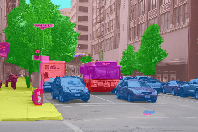
利用 StableDiffusionLDM3DPipeline 模型从提示词生成3D相关的图像(包括RGB图像和深度图像),并保存到指定路径。
- 通过 from_pretrained 方法从Hugging Face Model Hub加载预训练的 ldm3d-4c 模型。这个模型是特定于3D图像生成的稳定扩散模型。
- prompt: 定义生成图像时要使用的文本提示。name: 将生成的文件命名为“lemons”,以便后续保存时使用。
- 定义推理循环次数(iterations = 128),即模型将重复运行128次。在每次迭代中,通过 pipe(prompt) 使用提示词进行推理,返回结果包括 rgb_image 和 depth_image。计算推理总时间,并根据迭代次数计算平均延迟(每次推理所需的时间,单位为毫秒)和FPS(每秒帧数)。打印FPS,表示模型生成图像的速度。
- 生成的图像保存路径分别为RGB图像的 .jpg 文件和深度图像的 .png 文件。使用 save() 方法将图像保存到指定的文件路径中。
from diffusers import StableDiffusionLDM3DPipeline
import time
import torch
import intel_extension_for_pytorch as ipex # 引入Intel的PyTorch扩展
import os
# 加载模型
pipe = StableDiffusionLDM3DPipeline.from_pretrained("Intel/ldm3d-4c")
# 检查可用设备(xpu 或 CPU)
device = torch.device("xpu" if torch.xpu.is_available() else "cpu")
print(f"使用设备: {device}")
# 移到选择的设备
pipe.to(device)
# 定义提示词和输出名称
prompt = "A picture of some lemons on a table"
name = "lemons"
# 开始推理计时
t_start = time.time()
iterations = 128
# 模型推理
for _ in range(iterations):
output = pipe(prompt)
rgb_image, depth_image = output.rgb, output.depth
# 计算经过时间和 FPS
elapsed_time = time.time() - t_start
latency = elapsed_time / iterations * 1000 # 转换为毫秒
FPS = 1000 / latency
print(f"FPS: {FPS:.2f}")
# 指定输出路径
output_folder = "/home/dev/datasets"
# 确保输出文件夹存在
if not os.path.exists(output_folder):
os.makedirs(output_folder)
# 拼接完整的路径和文件名
rgb_image_path = os.path.join(output_folder, f"{name}_ldm3d_4c_rgb.jpg")
depth_image_path = os.path.join(output_folder, f"{name}_ldm3d_4c_depth.png")
# 保存图像
rgb_image[0].save(rgb_image_path)
depth_image[0].save(depth_image_path)
print(f"RGB 图像已保存至: {rgb_image_path}")
print(f"深度图像已保存至: {depth_image_path}")
结果
Loading pipeline components...: 100%|█████████████████████████████████████████████████████████████████████████████████████████████████████| 7/7 [00:00<00:00, 22.55it/s]
使用设备: xpu
100%|███████████████████████████████████████████████████████████████████████████████████████████████████████████████████████████████████| 49/49 [00:14<00:00, 3.39it/s]
...
100%|███████████████████████████████████████████████████████████████████████████████████████████████████████████████████████████████████| 49/49 [00:11<00:00, 4.20it/s]
FPS: 0.08
RGB 图像已保存至: /home/dev/datasets/lemons_ldm3d_4c_rgb.jpg
深度图像已保存至: /home/dev/datasets/lemons_ldm3d_4c_depth.png
生成的图像如下

深度图像生成如下

使用 Ernie 3.0 模型 进行推理,并且根据不同模式(GPU 或 TPU)来评估模型的性能,包括推理时间(延迟和帧率)以及模型的 FLOPs(浮点运算次数)和参数数量。
- GPU模式:检查 GPU 是否可用(XPU 设备),下载并加载 Ernie 3.0 模型,并将输入数据传输到设备。
- text: 需要输入的文本。max_length: 最大文本长度。model_path 和 tokenizer_path: 模型和分词器的路径。
- profile 函数通过 thop 库计算模型的 FLOPs(浮点运算次数)。计算模型的可训练参数数量,并将 FLOPs 转换为 GFLOPs(十亿次浮点运算)和参数数量转换为百万级别。
- 使用模型的前向传播函数 (self.model(**self.inputs)) 执行推理并返回输出。运行100次推理,计算平均延迟(latency)和帧率(FPS)。输出模型的 FLOPs 和参数量。
import os
import time
import torch
import intel_extension_for_pytorch as ipex # 引入Intel的PyTorch扩展
import requests
from transformers import BertTokenizer, ErnieModel
# from tpu_perf.infer import SGInfer
from thop import profile
import numpy as np
def download_model_weights(model_path):
if not os.path.exists(os.path.join(model_path, 'pytorch_model.bin')):
model_url = "https://huggingface.co/nghuyong/ernie-3.0-medium-zh/resolve/main/pytorch_model.bin?download=true"
response = requests.get(model_url)
if response.status_code == 200:
with open(os.path.join(model_path, 'pytorch_model.bin'), 'wb') as f:
f.write(response.content)
print("权重下载完成。")
else:
print("权重下载失败")
class ernie3:
def __init__(self, mode='gpu', text="Hello, how are you?", max_length=256, model_path='/home/dev/datasets/vocab', tokenizer_path='/home/dev/datasets/vocab'):
self.mode = mode
self.text = text
self.max_length = max_length
self.tokenizer_path = tokenizer_path
self.model_path = model_path
self.tokenizer = BertTokenizer.from_pretrained(tokenizer_path)
if mode == 'gpu':
self.device = torch.device("xpu" if torch.xpu.is_available() else "cpu")
download_model_weights(model_path)
self.model = ErnieModel.from_pretrained(model_path).to(self.device)
self.inputs = self.tokenizer(text=self.text, return_tensors='pt', padding='max_length', max_length=self.max_length).to(self.device)
elif mode == 'tpu':
self.inputs = self.tokenizer(text=text, return_tensors='pt', padding='max_length', max_length=max_length)
self.input_ids = self.inputs['input_ids'].numpy().astype(np.int32)
else:
raise ValueError("Mode should be either 'gpu' or 'tpu'")
def count_parameters_and_flops(self):
flops, _ = profile(self.model, (self.inputs.input_ids, self.inputs.attention_mask), verbose=False)
params = sum(p.numel() for p in self.model.parameters() if p.requires_grad)
return flops / 1e9 * 2, params / 1e6
def forward(self):
if self.mode == 'gpu':
outputs = self.model(**self.inputs)
return outputs
elif self.mode == 'tpu':
return self.input_ids
else:
raise ValueError("Mode should be either 'gpu' or 'tpu'")
#---------------------------------intel XPU测试-----------------------------------------------------
if __name__ == '__main__':
mode = 'gpu'
model = ernie3(mode=mode)
if mode == 'gpu':
iterations = 100
t_start = time.time()
for _ in range(iterations):
with torch.no_grad():
outputs = model.forward()
elapsed_time = time.time() - t_start
flops, params = model.count_parameters_and_flops()
latency = elapsed_time / iterations * 1000
FPS = 1000 / latency
print(f"FPS: {FPS:.2f}")
print(f"Latency: {latency:.2f} ms")
print(f"FLOPs: {flops} GFLOPs")
print(f"Parameters: {params} Million")
elif mode == 'tpu':
bmodel_path = "/home/aii-works/Benchmark/bmodel/language/nlp/ernie3/ernie3_1684x_f32.bmodel"
net = SGInfer(bmodel_path, devices=[0])
input = model.forward()
iterations = 100
t_start = time.time()
for _ in range(iterations):
output = net.infer_one(input)
elapsed_time = time.time() - t_start
latency = elapsed_time / iterations * 1000
FPS = 1000 / latency
print(f"FPS: {FPS:.2f}")
print(f"Latency: {latency:.2f} ms")
结果
FPS: 170.75
Latency: 5.86 ms
FLOPs: 21.764898816 GFLOPs
Parameters: 75.427584 Million
实现了用于生成文本的脚本,基于Hugging Face的Transformers库和Intel® Extension for PyTorch* (IPEX) 进行优化。它使用了GPT-2模型,并通过命令行参数来控制一些生成行为。
- 通过 argparse 来接受命令行参数。包括:dtype: 选择数据类型,可以是 float32 或 bfloat16,分别表示全精度和半精度浮点数。max-new-tokens: 生成的新tokens的最大数量。prompt: 输入的提示词,用于生成文本。greedy: 是否启用贪婪搜索,默认为 False,否则会使用beam search。batch-size: 生成文本时处理的批次大小。
- 根据 dtype 参数决定是否启用自动混合精度(AMP)。如果使用 bfloat16,则 amp_enabled 为 True,启用自动混合精度加速推理。
- 使用GPT-2模型,配置通过 AutoConfig 加载,并通过 AutoModelForCausalLM 加载模型的预训练权重。分词器 (tokenizer) 用于将自然语言转换为模型可以处理的输入格式。
- model.eval() 将模型设置为评估模式,禁用dropout等训练时特有的行为。channels_last 内存格式可以提升Intel硬件上的性能。ipex.llm.optimize 通过 Intel® Extension for PyTorch* 进一步优化模型的执行速度和内存使用。
- generate_kwargs 包含生成文本时的相关参数,如不进行采样 (do_sample=False),使用温度参数来控制文本生成的随机性。
- tokenizer 将输入提示 (prompt) 转换为token形式,并返回相应的张量。input_size 计算输入提示的token数量。提示被复制成多批次输入,用于处理多个输入(取决于 batch_size)。
- 使用 torch.inference_mode() 禁用梯度计算,以减少内存开销并加速推理。torch.cpu.amp.autocast 用于自动混合精度的推理(如果启用)。model.generate 根据输入提示生成新的文本,生成的长度由 max_new_tokens 参数控制。最后,通过 tokenizer.batch_decode 将生成的tokens解码为可读的文本,并打印生成结果及新增的token数量。
import torch
#################### code changes ####################
import intel_extension_for_pytorch as ipex
######################################################
import argparse
from transformers import (
AutoConfig,
AutoModelForCausalLM,
AutoTokenizer,
)
# args
parser = argparse.ArgumentParser("Generation script (fp32/bf16 path)", add_help=False)
parser.add_argument(
"--dtype",
type=str,
choices=["float32", "bfloat16"],
default="float32",
help="choose the weight dtype and whether to enable auto mixed precision or not",
)
parser.add_argument(
"--max-new-tokens", default=32, type=int, help="output max new tokens"
)
parser.add_argument(
"--prompt", default="What are we having for dinner?", type=str, help="input prompt"
)
parser.add_argument("--greedy", action="store_true")
parser.add_argument("--batch-size", default=1, type=int, help="batch size")
args = parser.parse_args()
print(args)
# dtype
amp_enabled = True if args.dtype != "float32" else False
amp_dtype = getattr(torch, args.dtype)
# load model
model_id = "gpt2" # 或者其他模型名称
config = AutoConfig.from_pretrained(
model_id, torchscript=True, trust_remote_code=True
)
model = AutoModelForCausalLM.from_pretrained(
model_id,
torch_dtype=amp_dtype,
config=config,
low_cpu_mem_usage=True,
trust_remote_code=True,
)
tokenizer = AutoTokenizer.from_pretrained(
model_id,
trust_remote_code=True
)
model = model.eval()
model = model.to(memory_format=torch.channels_last)
# Intel(R) Extension for PyTorch*
#################### code changes #################### # noqa F401
model = ipex.llm.optimize(
model,
dtype=amp_dtype,
inplace=True,
deployment_mode=True,
)
###################################################### # noqa F401
# generate args
num_beams = 1 if args.greedy else 4
generate_kwargs = dict(do_sample=False, temperature=0.9, num_beams=num_beams)
# input prompt
prompt = args.prompt
input_size = tokenizer(prompt, return_tensors="pt").input_ids.size(dim=1)
print("---- Prompt size:", input_size)
prompt = [prompt] * args.batch_size
# inference
with torch.inference_mode(), torch.cpu.amp.autocast(enabled=amp_enabled):
input_ids = tokenizer(prompt, return_tensors="pt").input_ids
gen_ids = model.generate(
input_ids,
max_new_tokens=args.max_new_tokens,
**generate_kwargs
)
gen_text = tokenizer.batch_decode(gen_ids, skip_special_tokens=True)
input_tokens_lengths = [x.shape[0] for x in input_ids]
output_tokens_lengths = [x.shape[0] for x in gen_ids]
total_new_tokens = [
o - i for i, o in zip(input_tokens_lengths, output_tokens_lengths)
]
print(gen_text, total_new_tokens, flush=True)
结果
['What are we having for dinner? What are we having for dinner? What are we having for dinner? What are we having for dinner? What are we having for dinner? What are we having'] [32]
使用 Intel Extension for PyTorch (IPEX) 来进行动态量化,对一个 BERT 模型进行动态量化处理,并将其转化为一个 TorchScript 模型保存下来。整个流程包括模型准备、量化、JIT 编译并使用 torch.jit.trace 和 torch.jit.freeze 来保存一个量化后的模型。
- 加载了预训练的 BertModel,这是一个来自 transformers 库的 BERT 模型,并将其设为推理模式(eval()),适合后续量化和推理。
- 生成了随机的输入数据,模拟了 BERT 模型的输入。vocab_size 是词汇表的大小,batch_size 是输入批次的大小,seq_length 是输入序列的长度。
- 使用 IPEX 提供的默认动态量化配置映射(qconfig_mapping)。动态量化是指只对模型的部分权重进行量化,而不对所有的权重和激活值进行静态量化。
- 通过 prepare 函数,模型被准备好进行动态量化。此过程将原始模型包装,添加量化所需的 observer 和 hooks。convert 函数将准备好的模型转换为量化的模型。经过转换后,模型内部的部分计算会使用更高效的量化运算。
- 使用 torch.jit.trace 对量化后的模型进行追踪,生成一个 TorchScript 模型。torch.jit.freeze 用来优化和冻结模型,确保未使用的部分不会在模型推理中引入不必要的开销。
- 将冻结的量化模型保存为 .pt 文件,可以用于后续的加载和推理。
import torch
#################### code changes #################### # noqa F401
import intel_extension_for_pytorch as ipex
from intel_extension_for_pytorch.quantization import prepare, convert
###################################################### # noqa F401
##### Example Model ##### # noqa F401
from transformers import BertModel
model = BertModel.from_pretrained("bert-base-uncased")
model.eval()
vocab_size = model.config.vocab_size
batch_size = 128
seq_length = 512
data = torch.randint(vocab_size, size=[batch_size, seq_length])
######################### # noqa F401
qconfig_mapping = ipex.quantization.default_dynamic_qconfig_mapping
# Alternatively, define your own qconfig:
# from torch.ao.quantization import PerChannelMinMaxObserver, PlaceholderObserver, QConfig, QConfigMapping
# qconfig = QConfig(
# activation = PlaceholderObserver.with_args(dtype=torch.float, is_dynamic=True),
# weight = PerChannelMinMaxObserver.with_args(dtype=torch.qint8, qscheme=torch.per_channel_symmetric))
# qconfig_mapping = QConfigMapping().set_global(qconfig)
prepared_model = prepare(model, qconfig_mapping, example_inputs=data)
converted_model = convert(prepared_model)
with torch.no_grad():
traced_model = torch.jit.trace(
converted_model, (data,), check_trace=False, strict=False
)
traced_model = torch.jit.freeze(traced_model)
traced_model.save("/home/dev/dynamic_quantized_model.pt")
print("Saved model to: dynamic_quantized_model.pt")
结果
Saved model to: dynamic_quantized_model.pt
算能 TPU 平台
TPU MLIR
技术栈架构
6.1.1 技术栈架构
-
系统软件层
- SOPHON设备驱动:为TPU提供基本的系统级支持(类似于NVIDIA GPU驱动)
- TPU-Kernel:基于SOPHON BM1684、BM1684X底层原子操作接口的底层编程接口(类似于CUDA Driver API)
- 需要用户熟悉设备硬件架构和指令集
- 提供与SOPHON TPU硬件交互的底层接口
- 适用于需要细粒度控制的高级应用
-
运行时环境层
- BMLib:提供基础接口,包括设备Handle管理、内存管理、数据搬运、API发送和同步等(类似于CUDA Runtime API的部分功能)
- BMRuntime:用于模型推理的运行时库(提供了类似CUDA Runtime API的高级抽象)
- 简化了TPU的使用
- 自动处理许多底层细节
-
编程模型和语言层
- BMLang:基于C++的面向SOPHON智能视觉深度学习处理器的高级编程库(类似于CUDA C/C++的角色)
- 使用张量数据(bmlang::Tensor)和计算操作(bmlang::Operator)编写代码
- 通过bmlang::compile或bmlang::compile_with_check生成可运行的BModel
- 支持在TPU和CPU上混合编程
- TPU-MLIR:支持将PyTorch、ONNX等框架模型转换为TOP MLIR,然后lowering到TPU MLIR,最后部署到BModel
- TPU-NNTC:支持多种框架模型的转换和量化,生成可在TPU上运行的BModel
- BMLang:基于C++的面向SOPHON智能视觉深度学习处理器的高级编程库(类似于CUDA C/C++的角色)
-
计算库层
- BMCV:提供张量运算及图像处理功能,如色彩空间转换、尺度变换、仿射变换等(类似于cuBLAS和其他CUDA专用算子库)
- SOPHON-MW:支持SOPHON设备硬件加速的多媒体库,包括SOPHON-OpenCV和SOPHON-FFmpeg
-
框架模型层
- SAIL (Sophon Artificial Intelligence Library):支持Python/C++的高级接口(类似于PyTorch和TensorFlow对CUDA的支持)
- 对BMRuntime、BMCV、sophon-mw等底层库接口的封装
- 简化了TPU编程,提供更高级的抽象
- PyTorch、TensorFlow等框架:通过TPU-MLIR或TPU-NNTC工具链支持这些框架模型的转换和优化,以在TPU上运行
- SAIL (Sophon Artificial Intelligence Library):支持Python/C++的高级接口(类似于PyTorch和TensorFlow对CUDA的支持)
总的来说,算能TPU的架构在很多方面与CUDA相似,都提供了从底层硬件接口到高级框架支持的完整堆栈。主要区别在于TPU更专注于深度学习处理器的优化,并提供了专门的模型编译和优化工具。
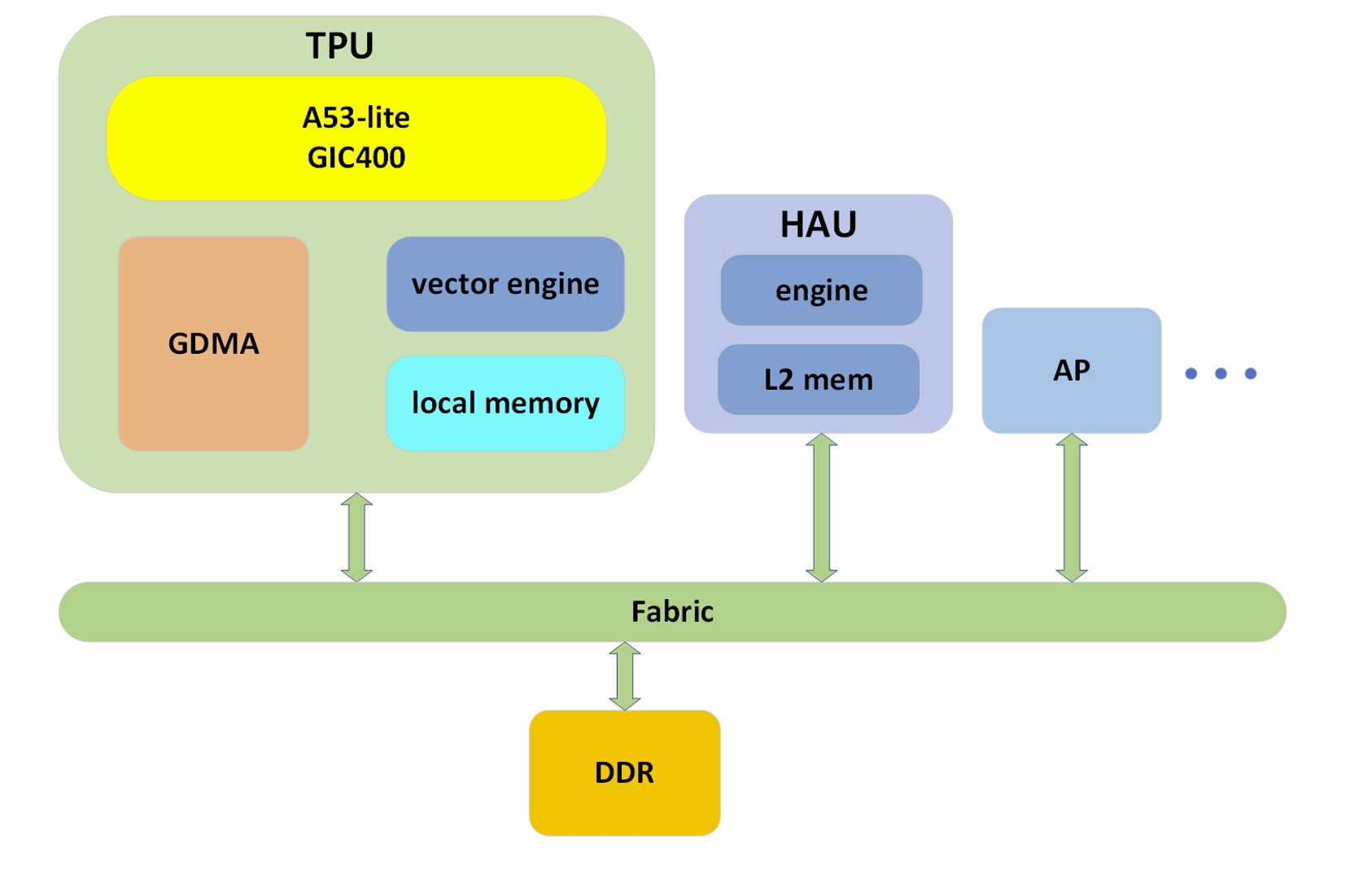 TPU(张量处理单元)是一种具有多个计算核心的架构设计,系统架构如图所示。TPU系统主要由TPU核心、L2 SRAM(L2内存)、片外DDR存储(全局内存)以及多个片间通信DMA(CDMA)等组件组成。在使用PPL进行编程时,用户直接与TPU核心进行交互。TPU采用标准的SIMD结构。Vector Engine中包含多个lane,每个lane中有若干个执行单元(EU)。每个EU相当于一个独立的计算单元,并且每个lane都有自己的局部内存,lane只能访问其专属的局部内存。在同一时刻,所有lane都执行相同的指令,EU进行相同类型的计算。
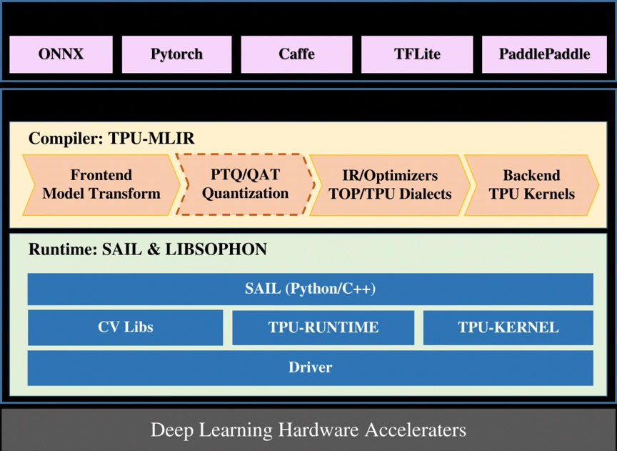
图片展示了算能TPU的软件栈架构,从顶层的深度学习框架到底层的硬件加速器,在图片中,SAIL位于中间层,作为运行时环境的一部分。而在AI技术栈中,SAIL被放在较高的"框架模型层"。这种差异反映了SAIL的多功能性:
- 作为运行时环境:SAIL提供了对底层硬件和库的封装,使其能够高效地执行编译后的模型。
- 作为高级接口:SAIL也提供了Python/C++的高级API,使开发者能够更容易地使用TPU的功能。
这种双重角色解释了为什么SAIL可以在不同的架构描述中出现在不同的层次。在实际应用中,SAIL既是连接高层框架和底层硬件的桥梁,也是开发者直接使用的高级接口。
系统软件层
Sophon软件框架与底层TPU的交互通常涉及多个层次和组件。
-
API和驱动层: Sophon软件框架提供了一系列API和驱动程序,这些程序用于与底层TPU硬件进行通信。这些API通常是高层的,便于用户调用。
-
模型编译: 在模型被训练后,需要将其转换为TPU可以理解的格式。这一过程通常涉及使用编译器(如MLIR或专用的模型编译工具),将深度学习模型转换为TPU优化的表示。
-
运行时环境: Sophon框架为TPU提供了一个运行时环境,负责管理TPU资源、调度任务并优化执行。在此环境中,TPU的计算资源被有效地分配给不同的任务。
-
调度与执行: 一旦模型被编译并加载到TPU上,运行时环境会负责调度执行。这包括管理数据传输、内存使用以及计算资源的调配,以确保高效的模型推理和训练。
-
数据传输: 数据在主机和TPU之间传输,通常通过高速接口(如PCIe)进行。这一过程需要优化,以减少延迟和带宽瓶颈。
-
性能优化: Sophon框架提供了一些性能优化技术,例如动态调度、张量融合等,来提升TPU的执行效率。
具体到Sophon Sail和BMRuntime,用户可以使用这些库来加载、运行模型,并通过特定的接口调用进行底层交互。
运行时环境层
展示了如何使用Sophon的sail库获取硬件设备的多种信息,包括TPU数量、利用率、温度、设备状态以及如何操作张量和进行数据编码。
- sophon.sail: 这是一个用于与Sophon硬件设备交互的库。通过该库,可以获取设备的状态、资源利用率和温度等信息。
- sail.get_available_tpu_num():获取当前可用的TPU数量,并将其存储在tpu_len变量中。
- dev_id设置为0,表示选择第一个设备。sail.get_vpp_util(dev_id):获取该设备的VPP(视频处理单元)利用率,并打印出来。
- sail.get_board_temp(dev_id):获取板卡的温度并打印。sail.get_chip_temp(dev_id):获取芯片的温度并打印。
- sail.get_dev_stat(dev_id):获取设备的状态信息并打印。
- sail.Handle(tpu_id):创建一个TPU句柄,用于后续的设备操作。handle.get_device_id():获取设备的ID。handle.get_sn():获取设备的序列号。handle.get_target():获取设备的目标信息。
- sail.Tensor(handle, input_data):将NumPy数组转换为Sophon张量。input_tensor1.shape():获取并打印张量的形状。arr.tobytes():将NumPy数组转换为字节格式。sail.base64_encode(handle, arr_bytes):将字节数据进行Base64编码。输出编码后的结果。
- sail.get_tpu_util(dev_id):获取指定设备的TPU利用率并打印。
import sophon.sail as sail
import numpy as np
if __name__ == '__main__':
# Get the number of available TPUs
tpu_len = sail.get_available_tpu_num()
print('Available TPU:', tpu_len)
# Get VPP utilization
dev_id = 0
print("VPP Utilization:", sail.get_vpp_util(dev_id))
# Get board temperature
print("Board Temperature:", sail.get_board_temp(dev_id))
# Get chip temperature
print("Chip Temperature:", sail.get_chip_temp(dev_id))
# Get device status
print("Device Status:", sail.get_dev_stat(dev_id))
# Create a Handle for TPU with ID 0
tpu_id = 0
handle = sail.Handle(tpu_id)
print("Device ID:", handle.get_device_id())
print("Serial Number:", handle.get_sn())
print("Target:", handle.get_target())
# Create a Tensor from a NumPy array
input_data = np.array([1, 2, 3])
input_tensor1 = sail.Tensor(handle, input_data)
print("Input Tensor Shape:", input_tensor1.shape())
# Convert a NumPy array to bytes and encode it
arr = np.array([[1, 2, 3], [4, 5, 6]])
arr_bytes = arr.tobytes()
base64_encoded_arr = sail.base64_encode(handle, arr_bytes)
print("Base64 Encoded Array:", base64_encoded_arr)
# Get TPU utilization
print("Device {} TPU Utilization is {} %".format(dev_id, sail.get_tpu_util(dev_id)))
结果
Available TPU: 1
VPP Utilization: [0, 0]
Board Temperature: 31
Chip Temperature: 37
Device Status: [14679, 0, 0]
Device ID: 0
Serial Number:
Target: BM1684X
Input Tensor Shape: [3]
Base64 Encoded Array: b'AQAAAAAAAAACAAAAAAAAAAMAAAAAAAAABAAAAAAAAAAFAAAAAAAAAAYAAAAAAAAA'
Device 0 TPU Utilization is 0 %
下面的代码结合了设备信息获取、处理器利用率、温度读取以及张量初始化等功能:
- 设备信息获取:使用 sail:Handle 对象获取设备 ID、序列号(SN)和目标信息。
- TPU 和 VPU 利用率:通过 sail:get_tpu_util 和 sail:get_vpu_util 函数分别获取 TPU 和 VPU 的使用率。
- 板和芯片温度:使用 sail:get_board_temp 和 sail:get_chip_temp 获取设备板和芯片的温度信息。
- 设备内存统计:调用 sail:get_dev_stat 获取设备的内存总量、已用内存以及 TPU 使用率。
- 张量初始化:通过 sail:Tensor 初始化两个张量对象,其中一个通过设备句柄进行初始化。
#include <stdio.h>
#include <sail/cvwrapper.h>
#include <iostream>
#include "tensor.h"
using namespace std;
int main() {
// Device initialization
int tpu_id = 0;
sail::Handle handle(tpu_id);
// Print basic device information
std::cout << "Device ID: " << handle.get_device_id() << std::endl;
std::cout << "SN: " << handle.get_sn() << std::endl;
std::cout << "Target: " << handle.get_target() << std::endl;
// Get TPU utilization
int tpu_util = sail::get_tpu_util(0);
std::cout << "TPU Utilization: " << tpu_util << "%" << std::endl;
// Get VPU utilization
std::vector<int> vpu_util = sail::get_vpu_util(0);
for(int i = 0; i < vpu_util.size(); i++) {
std::cout << "VPU ID: " << i << ", Utilization: " << vpu_util[i] << "%" << std::endl;
}
// Get board temperature
int board_temp = sail::get_board_temp(0);
std::cout << "Board Temperature: " << board_temp << "℃" << std::endl;
// Get chip temperature
int chip_temp = sail::get_chip_temp(0);
std::cout << "Chip Temperature: " << chip_temp << "℃" << std::endl;
// Get device memory statistics
std::vector<int> dev_stat = sail::get_dev_stat(0);
std::cout << "Memory Total: " << dev_stat[0] << " MB" << std::endl;
std::cout << "Memory Used: " << dev_stat[1] << " MB" << std::endl;
std::cout << "TPU Utilization: " << dev_stat[2] << " %" << std::endl;
// Tensor initialization
int dev_id = 0;
sail::Handle tensor_handle(dev_id);
std::shared_ptr<sail::Tensor> input_tensor1, input_tensor2;
std::vector<int> input_shape = {10, 10};
bm_data_type_t input_dtype = BM_FLOAT32; // dtype can be BM_FLOAT32, BM_INT8, etc.
// Initialize tensors
input_tensor1 = std::make_shared<sail::Tensor>(input_shape, input_dtype);
input_tensor2 = std::make_shared<sail::Tensor>(tensor_handle, input_shape, input_dtype, true, true);
return 0;
}
编程模型和语言层
TPU-MLIR 介绍
TPU-MLIR 是算能深度学习处理器的编译器工程,提供了一套完整的工具链,用于将不同框架下预训练的神经网络转化为可以在算能智能视觉深度学习处理器上高效运行的模型文件(BModel/CviModel)。
主要特点
- 支持多种框架:直接支持 PyTorch、ONNX、TFLite 和 Caffe 等框架模型的转换。
- 开源:代码已开源到 GitHub(https://github.com/sophgo/tpu-mlir)。
- 学术支持:有相关论文描述其整体设计思路(https://arxiv.org/abs/2210.15016)。
架构概览
TPU-MLIR 的整体架构包括以下主要组件:
- 前端转换:将各种框架的模型转换为 MLIR 表示。
- 优化阶段:对 MLIR 进行各种优化。
- 后端生成:生成可在 TPU 上运行的 BModel/CviModel。
使用流程
1. 模型转换
使用 model_transform 工具将原始模型转换成 MLIR 文件。
2. 量化(可选)
如需 INT8 量化:
- 使用
run_calibration生成校准表。 - 使用
run_qtable生成量化表(用于决定哪些层采用浮点计算)。
3. 模型部署
使用 model_deploy 将 MLIR 文件转换成 BModel/CviModel。
Lowering 过程
TPU-MLIR使用两种主要的方言:TOP(Tensor Operator)和TPU。
-
TOP方言:
- 硬件无关层
- 支持F32/F16/BF16/INT8对称/INT8非对称等类型
- 代表了网络的高级表示
-
TPU方言:
- 硬件相关层
- 针对特定TPU硬件优化
- 包含了硬件特定的量化和优化策略
Lowering是将TOP层OP下沉到TPU层OP的过程:
-
将算子从硬件无关层(TOP)转换到硬件相关层(TPU)
-
支持F32/F16/BF16/INT8对称/INT8非对称等类型转换
-
涉及量化算法,针对不同硬件有不同实现
-
处理混合精度情况,在需要时插入CastOp Lowering 是将 TOP 层 OP 下沉到 TPU 层 OP 的过程:
-
支持 F32/F16/BF16/INT8 对称/INT8 非对称等类型转换
-
处理混合精度情况,在需要时插入 CastOp
CodeGen 过程
CodeGen 是将 MLIR 文件转换为最终 BModel 的过程,主要包括:
- 指令生成:执行不同 op 的 CodeGen 接口,生成相应的二进制指令
- 指令存储:使用 store_cmd 将指令存储在指定数据结构中
- 指令取出:所有 op 的二进制码生成完毕后,调用 BM168X 系列类中封装的函数取出指令,最终生成 BModel
后端实现
- 使用动态库(libbackend_xxx.so)封装硬件后端
- 通过函数指针加载后端函数
- 使用 EngineStorer 和 CmdStorer 系列类管理指令存储
- 采用单例模式和装饰器模式实现灵活的指令管理
通过这种设计,TPU-MLIR 能够有效地将各种深度学习框架的模型转换为可在 TPU 上高效运行的 BModel,同时提供了灵活的优化和定制空间。
自定义算子开发
TPU-MLIR 支持添加自定义算子,主要步骤如下:
1. 前端定义
使用 TpuLang 接口定义自定义算子:
import transform.TpuLang as tpul
tpul.init("BM1684X", True)
# 定义输入
x = tpul.Tensor(dtype="float32", shape=[1, 3, 224, 224], name="input")
# 添加自定义算子
def shape_func(tensors_in):
return [tensors_in[0].shape]
outs = tpul.custom(
tensors_in=[x],
shape_func=shape_func,
op_name="custom_op_name",
params={"param1": value1, "param2": value2},
out_dtypes=["float32"],
out_names=["custom_out"]
)
# 编译生成 MLIR
tpul.compile("model_name", [x], outs, False, 2, has_custom=True)
2. 后端实现
- 在
$TPUC_ROOT/customlayer/include添加头文件。 - 在
$TPUC_ROOT/customlayer/src添加实现文件。 - 在
backend_custom_param.h定义参数结构体。 - 添加 API 接口文件。
- 在
backend_custom_api.cpp定义后端调用接口。 - 运行
$TPUC_ROOT/customlayer/build.sh编译生成动态库。
TPU-MLIR 提供了一个强大的工具链,支持从多种深度学习框架到 TPU 可执行模型的转换。通过支持自定义算子,它为开发者提供了极大的灵活性,使得复杂的深度学习模型能够在 TPU 上高效运行。结合 TPUPerf 工具,开发者可以全面优化和验证其模型性能。
TPU平台专门支持BModel模型加速,因此在使用TPU之前,必须进行模型迁移。通过利用MLIR工具链,可以将在其他框架中训练的模型转换为BModel,从而实现TPU的兼容运行。
MLIR已经直接支持绝大多数开源框架(如Pytorch、ONNX、TFLite和Caffe)中的算子和模型,而对于其他框架(如TensorFlow和PaddlePaddle),则需要先将其转换为ONNX模型,然后再进行后续转换。这一过程的整体架构可以参见TPU-MLIR工具链示意图。
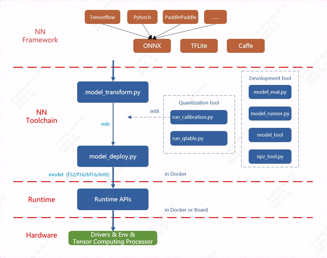 模型转换主要包括两个步骤。首先,通过
 model_transform.py 脚本将原始模型转换为 MLIR 文件。然后,使用 model_deploy.py 脚本将生成的 MLIR 文件转换为 BModel。
在生成浮点型模型时,model_deploy.py 工具支持输出三种不同的浮点数据类型:F32、F16 和 BF16。而对于 INT8 模型,首先需要准备一个量化数据集,并调用 run_calibration.py 生成校准表。接着,将校准表传递给 model_deploy.py 以完成 INT8 模型的生成。
如果生成的 INT8 模型精度不符合要求,可以使用 run_qtable.py 工具生成量化表,量化表用于决定哪些网络层使用浮点计算,随后将该量化表传递给 model_deploy.py,以生成混合精度模型。
以 yolov5s.onnx 为例, 介绍如何编译迁移一个onnx模型至BM1684X 平台运行。
在与 tpu-mlir 同级的目录下创建一个名为 model_yolov5s 的目录,并将模型文件和图片文件都放入该目录。具体步骤如下:
-
进入正确的父目录**:确保位于与
tpu-mlir同级的目录中。例如:cd /path/to/your/parent_directory -
创建
model_yolov5s目录:mkdir model_yolov5s -
将模型文件和COCO2017数据集图片文件复制到新建的
model_yolov5s目录中:cp /path/to/your/model_file /path/to/your/image_file ./model_yolov5s/确保将模型文件(例如
.pt、.onnx、.mlir等格式的文件)和图片文件(例如.jpg、.png等格式的图片)都放入model_yolov5s目录中。 完成后,目录结构应该类似于以下形式:
/parent_directory
├── tpu-mlir
└── model_yolov5s
├── your_model_file
└── your_image_file
如果模型的输入是图片格式,在进行模型转换前,必须先了解并执行必要的预处理操作。然而,如果模型输入的是已经经过预处理的 npz 文件,则无需再进行额外的预处理步骤。在官方的 YOLOv5 模型中,图片输入采用 RGB 格式,并且每个像素值都会乘以 1/255 进行归一化处理。这相当于将每个像素的值缩放至 0 到 1 之间。对应地,转换时的 mean(均值)为 [0.0, 0.0, 0.0],而 scale(缩放系数)为 [0.0039216, 0.0039216, 0.0039216],因为 1/255 等于 0.0039216。 模型转换命令如下:
$ model_transform.py \
--model_name yolov5s \
--model_def ../yolov5s.onnx \
--input_shapes [[1,3,640,640]] \
--mean 0.0,0.0,0.0 \
--scale 0.0039216,0.0039216,0.0039216 \
--keep_aspect_ratio \
--pixel_format rgb \
--output_names 350,498,646 \
--test_input ../image/dog.jpg \
--test_result yolov5s_top_outputs.npz \
--mlir yolov5s.mlir
在模型转换为 MLIR 文件后,会生成一个名为 ${model_name}_in_f32.npz 的文件。该文件包含模型的输入数据,以 .npz 格式存储,通常用于模型推理时作为输入文件,确保数据格式与模型的输入要求一致。
将 MLIR 文件转换为 F32 格式的 BModel,操作步骤如下:
$ model_deploy.py \
--mlir yolov5s.mlir \
--quantize F32 \
--chip bm1684x \
--test_input yolov5s_in_f32.npz \
--test_reference yolov5s_top_outputs.npz \
--tolerance 0.99,0.99 \
--model yolov5s_1684x_f32.bmodel
编译完成后, 会生成名为 yolov5s_1684x_f32.bmodel 的文件。 将 MLIR 文件转换为 F16 格式的 BModel,具体操作步骤如下:
$ model_deploy.py \
--mlir yolov5s.mlir \
--quantize F16 \
--chip bm1684x \
--test_input yolov5s_in_f32.npz \
--test_reference yolov5s_top_outputs.npz \
--model yolov5s_1684x_f16.bmodel
编译完成后, 会生成名为 yolov5s_1684x_f16.bmodel 的文件。 在转换为 INT8 模型之前,首先需要运行校准过程(calibration)来生成校准表。校准过程中,输入的数据数量根据具体需求准备,通常在 100 到 1000 张图片左右。
生成校准表后,可以选择生成对称或非对称的 BModel。如果对称模型能满足需求,通常不建议使用非对称模型,因为非对称模型的性能会稍逊于对称模型。
以下是使用现有的 100 张来自 COCO2017 数据集的图片作为示例,执行校准的步骤:
-
准备校准数据集:确保已经准备好 100 张 COCO2017 的图片,并将其放置在指定的目录中。
-
运行校准命令:通过以下命令运行校准,生成校准表:
$ run_calibration.py yolov5s.mlir \
--dataset ../COCO2017 \
--input_num 100 \
-o yolov5s_cali_table
- 生成 INT8 模型:使用生成的校准表,执行以下命令,将校准表传递给
model_deploy.py以生成对称或非对称的 INT8 BModel:
$ model_deploy.py \
--mlir yolov5s.mlir \
--quantize INT8 \
--calibration_table yolov5s_cali_table \
--chip bm1684x \
--test_input yolov5s_in_f32.npz \
--test_reference yolov5s_top_outputs.npz \
--tolerance 0.85,0.45 \
--model yolov5s_1684x_int8_sym.bmodel
如果对称模型能够满足精度要求,通常选择对称模式,因为它的性能表现优于非对称模型。编译完成后, 会生成名为 yolov5s_1684x_int8_sym.bmodel 的文件。
效果检验
完成目标检测的整个流程,包括数据预处理、推理、后处理(NMS)和结果的可视化。
- 图像预处理:将输入图像缩放到模型接受的尺寸。
- 推理:调用 mlir_inference 或 onnx_inference 等模型推理函数,得到检测结果。
- 后处理:通过 postproc 函数解析模型输出,结合锚点生成预测框和类别。
- NMS:通过 multiclass_nms 函数对预测框进行非极大值抑制,过滤冗余框。
- 可视化:使用 vis 函数将检测结果绘制到图像上,展示检测出的物体和对应类别。 部分重要代码如下:
import numpy as np
import cv2
COCO_CLASSES = ("person", "bicycle", "car", "motorcycle", "airplane", "bus", "train", "truck", ...)
_COLORS = np.array([...]).astype(np.float32).reshape(-1, 3)
ANCHORS = {8: [[1.25, 1.625], [2.0, 3.75], [4.125, 2.875]], ...}
def vis(img, boxes, scores, cls_ids, conf=0.5, class_names=None):
for i in range(len(boxes)):
if scores[i] < conf: continue
box, cls_id = boxes[i], int(cls_ids[i])
color = (_COLORS[cls_id] * 255).astype(np.uint8).tolist()
text = '{}:{:.1f}%'.format(class_names[cls_id], scores[i] * 100)
cv2.rectangle(img, (int(box[0]), int(box[1])), (int(box[2]), int(box[3])), color, 1)
cv2.putText(img, text, (int(box[0]), int(box[1])), cv2.FONT_HERSHEY_SIMPLEX, 0.4, (0, 0, 0), 1)
return img
def nms(boxes, scores, iou_thres):
x1, y1, x2, y2 = boxes[:, 0], boxes[:, 1], boxes[:, 2], boxes[:, 3]
areas = (x2 - x1 + 1) * (y2 - y1 + 1)
order = scores.argsort()[::-1]
keep = []
while order.size > 0:
i = order[0]
keep.append(i)
xx1 = np.maximum(x1[i], x1[order[1:]])
yy1 = np.maximum(y1[i], y1[order[1:]])
xx2 = np.minimum(x2[i], x2[order[1:]])
yy2 = np.minimum(y2[i], y2[order[1:]])
inter = np.maximum(0.0, xx2 - xx1 + 1) * np.maximum(0.0, yy2 - yy1 + 1)
ovr = inter / (areas[i] + areas[order[1:]] - inter)
order = order[np.where(ovr <= iou_thres)[0] + 1]
return keep
def multiclass_nms(boxes, scores, iou_thres, score_thres, class_agnostic=False):
if class_agnostic:
cls_inds, cls_scores = scores.argmax(1), scores.max(1)
else:
final_dets, num_classes = [], scores.shape[1]
for cls_ind in range(num_classes):
valid_mask = scores[:, cls_ind] > score_thres
if valid_mask.sum() > 0:
keep = nms(boxes[valid_mask], scores[valid_mask, cls_ind], iou_thres)
if keep: final_dets.append(np.hstack([boxes[valid_mask][keep], scores[valid_mask][keep, None], np.full((len(keep), 1), cls_ind)]))
return np.vstack(final_dets) if final_dets else None
def preproc(img, input_size):
r = min(input_size[0] / img.shape[0], input_size[1] / img.shape[1])
resized_img = cv2.resize(img, (int(img.shape[1] * r), int(img.shape[0] * r)), interpolation=cv2.INTER_LINEAR)
padded_img = np.ones(input_size + (3,), dtype=np.uint8) * 114
padded_img[:resized_img.shape[0], :resized_img.shape[1]] = resized_img
return np.ascontiguousarray(padded_img.transpose((2, 0, 1)), dtype=np.float32), r
def make_grid(nx, ny, stride, anchor):
return np.stack(np.meshgrid(np.arange(nx), np.arange(ny)), -1), np.array(anchor).reshape(1, len(anchor), 1, 1, 2)
用以上代码分别来验证onnx/f16/f32的执行结果。 onnx模型的执行方式如下, 得到 dog_onnx.jpg :
$ detect_yolov5.py \
--input ../image/dog.jpg \
--model ../yolov5s.onnx \
--output dog_onnx.jpg
f16 bmodel的执行方式如下, 得到 dog_f16.jpg :
$ detect_yolov5.py \
--input ../image/dog.jpg \
--model yolov5s_1684x_f16.bmodel \
--output dog_f16.jpg
int8对称bmodel的执行方式如下, 得到 dog_f32.jpg :
$ detect_yolov5.py \
--input ../image/dog.jpg \
--model yolov5s_1684x_f32.bmodel \
--output dog_f32.jpg
dog_onnx.jpg:
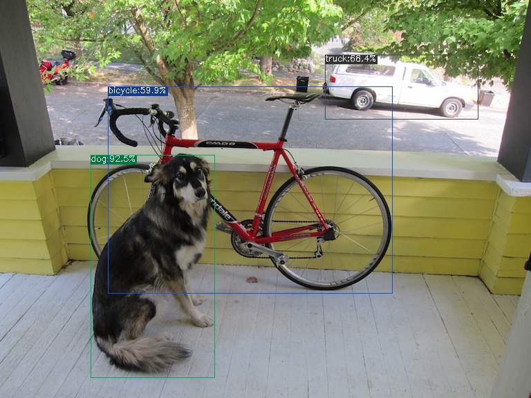
dog_f16.jpg:

dog_f32.jpg:

性能分析
通过利用Profile数据和TPU Profile工具,可以可视化模型的完整运行流程,从而便于进行性能分析。首先,将生成的yolov5s_bm1684x_f16.bmodel文件复制到已安装libsophon的运行环境中。与编译过程类似,运行时的Profile功能默认是关闭的,以避免在保存和传输Profile时造成额外的时间消耗。当需要启用Profile功能时,只需在运行编译好的bmodel之前设置环境变量BMRUNTIME_ENABLE_PROFILE=1。然后,使用libsophon提供的模型测试工具bmrt_test运行bmodel,以生成Profile数据。
# 通过环境变量(BMRUNTIME_ENABLE_PROFILE)使能profile, 生成二进制数据
BMRUNTIME_ENABLE_PROFILE=1 bmrt_test --bmodel resnet50_fix8b.bmodel
结果
[BMRT][load_bmodel:1734] INFO:pre net num: 0, load net num: 1
[BMRT][load_tpu_module:1830] INFO:loading firmare in bmodel
[BMRT][preload_funcs:2149] INFO: core_id=0, multi_fullnet_func_id=148
[BMRT][preload_funcs:2152] INFO: core_id=0, dynamic_fullnet_func_id=149
[BMRT][setup_profile_context:814] WARNING:bmodel do not contain any profile info
[BMRT][show_net_info:2535] INFO: ########################
[BMRT][show_net_info:2540] INFO: NetName: yolov5s, Index=0, CoreNum=1
[BMRT][show_net_info:2543] INFO: ---- stage 0 ----
[BMRT][show_net_info:2553] INFO: Input 0) 'images' shape=[ 1 3 640 640 ] dtype=FLOAT32 scale=1 zero_point=0 device_id=0
[BMRT][show_net_info:2564] INFO: Output 0) 'output_Concat' shape=[ 1 25200 85 ] dtype=FLOAT32 scale=1 zero_point=0 device_id=0
[BMRT][show_net_info:2564] INFO: Output 1) '350_Transpose' shape=[ 1 3 80 80 85 ] dtype=FLOAT32 scale=1 zero_point=0 device_id=0
[BMRT][show_net_info:2564] INFO: Output 2) '498_Transpose' shape=[ 1 3 40 40 85 ] dtype=FLOAT32 scale=1 zero_point=0 device_id=0
[BMRT][show_net_info:2564] INFO: Output 3) '646_Transpose' shape=[ 1 3 20 20 85 ] dtype=FLOAT32 scale=1 zero_point=0 device_id=0
[BMRT][show_net_info:2567] INFO: ########################
[BMRT][bmrt_test:889] INFO:==> running network #0, name: yolov5s, loop: 0
[BMRT][bmrt_test:944] INFO:reading input #0, bytesize=4915200
[BMRT][print_array:756] INFO: --> input_data: < 0 0 0 0 0 0 0 0 0 0 0 0 0 0 0 0 ... > len=1228800
[BMRT][write_block:324] INFO: write_block: type=1, len=36
[BMRT][write_block:324] INFO: write_block: type=8, len=44
[BMRT][end:76] INFO:bdc record_num=2189, max_record_num=1048576
[BMRT][write_block:324] INFO: write_block: type=3, len=70048
[BMRT][end:89] INFO:gdma record_num=321, max_record_num=1048576
[BMRT][write_block:324] INFO: write_block: type=4, len=61632
[BMRT][write_block:324] INFO: write_block: type=5, len=288
[BMRT][write_block:324] INFO: write_block: type=6, len=1340
[BMRT][print_note:100] INFO:*****************************************************************
[BMRT][print_note:101] INFO:* PROFILE MODE due to BMRUNTIME_ENABLE_PROFILE=1
[BMRT][print_note:102] INFO:* Note: BMRuntime will collect time data during running *
[BMRT][print_note:103] INFO:* that will cost extra time. *
[BMRT][print_note:104] INFO:* Close PROFILE Mode by "unset BMRUNTIME_ENABLE_PROFILE"
[BMRT][print_note:105] INFO:*****************************************************************
[BMRT][bmrt_test:1089] INFO:reading output #0, bytesize=8568000
[BMRT][print_array:756] INFO: --> output ref_data: < 0 0 0 0 0 0 0 0 0 0 0 0 0 0 0 0 ... > len=2142000
[BMRT][bmrt_test:1089] INFO:reading output #1, bytesize=6528000
[BMRT][print_array:756] INFO: --> output ref_data: < 0 0 0 0 0 0 0 0 0 0 0 0 0 0 0 0 ... > len=1632000
[BMRT][bmrt_test:1089] INFO:reading output #2, bytesize=1632000
[BMRT][print_array:756] INFO: --> output ref_data: < 0 0 0 0 0 0 0 0 0 0 0 0 0 0 0 0 ... > len=408000
[BMRT][bmrt_test:1089] INFO:reading output #3, bytesize=408000
[BMRT][print_array:756] INFO: --> output ref_data: < 0 0 0 0 0 0 0 0 0 0 0 0 0 0 0 0 ... > len=102000
[BMRT][bmrt_test:1139] INFO:net[yolov5s] stage[0], launch total time is 271429 us (npu 20523 us, cpu 250906 us), (launch func time 271425 us, sync 4 us)
[BMRT][bmrt_test:1146] INFO:+++ The network[yolov5s] stage[0] output_data +++
[BMRT][print_array:756] INFO:output data #0 shape: [1 25200 85 ] < 5.22443 2.85089 10.7558 10.5032 6.54244e-06 0.176123 0.00520219 0.044946 0.0045222 0.00351634 0.00180591 0.0015516 0.00476113 0.00907193 0.0473877 0.00191117 ... > len=2142000
[BMRT][print_array:756] INFO:output data #1 shape: [1 3 80 80 85 ] < 0.308533 -0.289279 0.0742412 -0.202984 -11.9372 -1.54284 -5.25346 -3.05631 -5.39422 -5.64681 -6.31488 -6.46692 -5.3425 -4.69346 -3.00084 -6.25813 ... > len=1632000
[BMRT][print_array:756] INFO:output data #2 shape: [1 3 40 40 85 ] < -0.0399987 0.252585 -0.383008 -0.521117 -11.0394 -1.3127 -5.11408 -3.31933 -5.46268 -5.97731 -5.76262 -6.10796 -5.14695 -5.37918 -2.57402 -6.29721 ... > len=408000
[BMRT][print_array:756] INFO:output data #3 shape: [1 3 20 20 85 ] < 0.714055 0.655423 -0.535399 -0.240734 -9.81843 -1.2305 -5.77227 -3.35369 -5.92415 -5.12047 -5.79011 -5.18393 -5.22128 -5.52896 -4.52387 -6.63506 ... > len=102000
[BMRT][bmrt_test:1208] INFO:load input time(s): 0.003325
[BMRT][bmrt_test:1209] INFO:pre alloc time(s): 0.000004
[BMRT][bmrt_test:1210] INFO:calculate time(s): 0.271429
[BMRT][bmrt_test:1211] INFO:get output time(s): 0.004142
[BMRT][bmrt_test:1212] INFO:compare time(s): 0.001548
结果可视化
将上述步骤生成的bmprofile_data-1目录复制回Docker中的tpu-mlir工程环境。tpu-mlir提供了tpu_profile脚本,用于将生成的二进制Profile数据转换为网页文件并进行可视化。在Docker内执行以下命令:
tpu_profile bmprofile_data-1 bmprofile_out
ls bmprofile_out
# echarts.min.js profile_data.js result.html
执行命令后会生成bmprofile_out文件夹,在浏览器中打开bmprofile_out/result.html,即可查看Profile的图表。
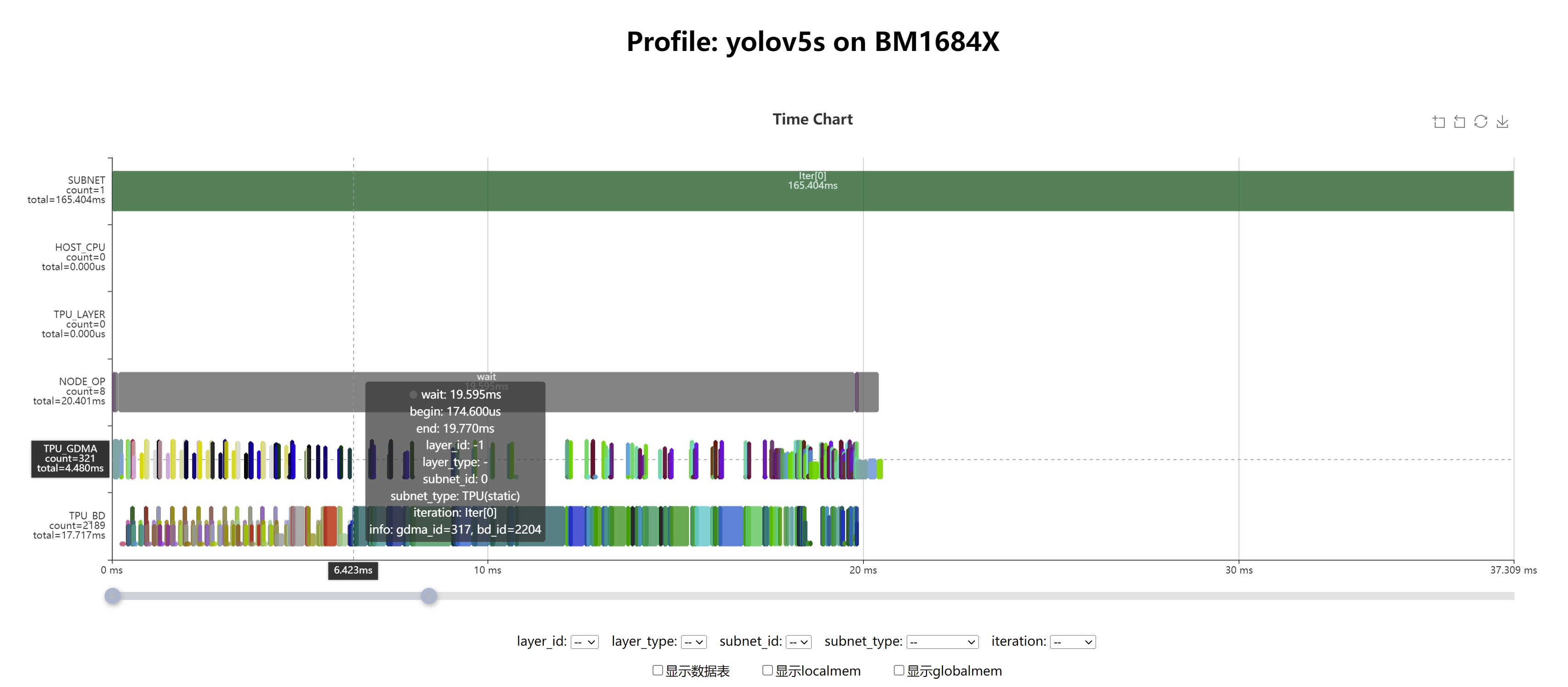
计算库层
C++计算库
以算法的执行为例,按照算法的执行先后顺序展开介绍:
1.加载bmodel模型
2.预处理
3.推理
加载bmodel模型
首先是加载 bmodel 模型、管理 bmruntime 的初始化、提取网络信息,并为模型推理阶段准备输入输出张量。
- 构造函数 BMNNContext:这是一个类的构造函数,用于初始化类实例。它接收一个 BMNNHandlePtr 类型的句柄 handle 和一个字符串指针 bmodel_file,代表要加载的 bmodel 文件路径。m_handlePtr(handle):将传入的 handle 赋值给类成员 m_handlePtr。bm_handle_t hdev = m_handlePtr->handle();:通过句柄获取硬件设备句柄 hdev。bmrt_create(hdev):基于设备句柄创建 bmruntime 上下文对象。若创建失败,会打印错误信息并退出。bmrt_load_bmodel:从指定的 bmodel 文件中加载模型。如果失败,输出错误信息。load_network_names():调用该函数来加载网络的名字。
- bmrt_get_network_number:获取当前 bmodel 中包含的网络数量。bmrt_get_network_names:获取所有网络的名称,保存在 names 中。m_network_names.push_back(names[i]):将网络名称保存到类成员变量 m_network_names 的容器中。free(names):释放 names 指针的内存。
- BMNNNetwork 构造函数:通过模型名称 name 来创建一个网络实例,并初始化相关的张量。bmrt_get_bm_handle(bmrt):获取 bmruntime 的设备句柄,并将其转换为 bm_handle_t 类型。bmrt_get_network_info:通过模型名称获取该模型的详细信息,存储在 m_netinfo 中。m_max_batch:用来记录模型支持的最大批次。batches.push_back:遍历所有的阶段,获取输入形状的第一个维度(通常是批次大小),并将其添加到批次列表中。记录最大的批次大小。m_inputTensors 和 m_outputTensors:分别为输入和输出张量分配内存空间。张量初始化:为每个输入张量设置数据类型(dtype)、形状(shape)、存储模式(st_mode),并将其初始化为空的设备内存。
BMNNContext(BMNNHandlePtr handle, const char* bmodel_file):m_handlePtr(handle){
bm_handle_t hdev = m_handlePtr->handle();
// init bmruntime contxt
m_bmrt = bmrt_create(hdev);
if (NULL == m_bmrt) {
std::cout << "bmrt_create() failed!" << std::endl;
exit(-1);
}
// load bmodel from file
if (!bmrt_load_bmodel(m_bmrt, bmodel_file)) {
std::cout << "load bmodel(" << bmodel_file << ") failed" << std::endl;
}
load_network_names();
}
...
void load_network_names() {
const char **names;
int num;
// get network info
num = bmrt_get_network_number(m_bmrt);
bmrt_get_network_names(m_bmrt, &names);
for(int i=0;i < num; ++i) {
m_network_names.push_back(names[i]);
}
free(names);
}
...
BMNNNetwork(void *bmrt, const std::string& name):m_bmrt(bmrt) {
m_handle = static_cast<bm_handle_t>(bmrt_get_bm_handle(bmrt));
// get model info by model name
m_netinfo = bmrt_get_network_info(bmrt, name.c_str());
m_max_batch = -1;
std::vector<int> batches;
for(int i=0; i<m_netinfo->stage_num; i++){
batches.push_back(m_netinfo->stages[i].input_shapes[0].dims[0]);
if(m_max_batch<batches.back()){
m_max_batch = batches.back();
}
}
m_batches.insert(batches.begin(), batches.end());
m_inputTensors = new bm_tensor_t[m_netinfo->input_num];
m_outputTensors = new bm_tensor_t[m_netinfo->output_num];
for(int i = 0; i < m_netinfo->input_num; ++i) {
// get data type
m_inputTensors[i].dtype = m_netinfo->input_dtypes[i];
m_inputTensors[i].shape = m_netinfo->stages[0].input_shapes[i];
m_inputTensors[i].st_mode = BM_STORE_1N;
m_inputTensors[i].device_mem = bm_mem_null();
}
...
- FFALIGN(m_net_w, 64):这行代码用于对 m_net_w(网络的宽度)进行64字节对齐。FFALIGN 函数通常用于确保内存地址或大小是指定字节的倍数,以便提高内存访问的效率。
aligned_net_w:对齐后的网络宽度。
}
预处理
代码首先对网络的宽度进行64字节对齐,以确保高效的内存访问。然后根据对齐后的宽度创建图像对象,用于存储推理结果和推理输入。 图像对象的内存分配是连续的,确保批处理时数据在内存中紧凑排列,减少内存碎片。数据类型处理:根据模型的输入数据类型(FP32 或 INT8),动态调整输入图像的存储格式,保证图像数据与推理需求匹配。
- FFALIGN(m_net_w, 64):这行代码用于对 m_net_w(网络的宽度)进行64字节对齐。FFALIGN 函数通常用于确保内存地址或大小是指定字节的倍数,以便提高内存访问的效率。 aligned_net_w:对齐后的网络宽度。
- bm_image_create:为每个批次创建 bm_image 对象。此函数将生成 max_batch 数量的图像对象,每个图像的尺寸为 m_net_h x m_net_w,格式为 FORMAT_RGB_PLANAR,数据类型为 DATA_TYPE_EXT_1N_BYTE(1字节无符号整数)。m_resized_imgs[i]:图像数组中的每个元素将用于存储推理结果。strides:使用上面定义的步长数组,确保每个通道数据的对齐。assert(BM_SUCCESS == ret):检查图像创建是否成功,若不成功则程序将终止。
- bm_image_alloc_contiguous_mem:为 m_resized_imgs 数组中的图像分配连续的内存。这样做的好处是,多个图像共享同一段连续的内存区域,这可能会提高推理和数据传输的效率,尤其在批量处理时。max_batch:一次为所有批次的图像分配内存。m_resized_imgs.data():提供图像数组的起始地址。
- bm_image_data_format_ext img_dtype:定义输入图像的格式,这里初始为 DATA_TYPE_EXT_FLOAT32,表示数据类型为 32 位浮点数。if (tensor->get_dtype() == BM_INT8):检查模型输入的张量类型。如果张量的数据类型为 BM_INT8(8位整型),则将 img_dtype 修改为 DATA_TYPE_EXT_1N_BYTE_SIGNED(1字节有符号整数)。这一步是根据推理引擎支持的输入数据类型动态调整图像的存储格式。
- bm_image_create_batch:用于创建一个批次的 bm_image 对象,所有批次的图像共用同样的格式和大小:m_net_h, m_net_w:图像的高度和宽度。FORMAT_RGB_PLANAR:图像格式为分离的 RGB 通道。img_dtype:图像的实际数据类型(根据推理需求为 FP32 或 INT8)。m_converto_imgs.data():用于存储批次图像的数组。max_batch:批次大小,即一次推理的输入图像数量。
int aligned_net_w = FFALIGN(m_net_w, 64);
int strides[3] = {aligned_net_w, aligned_net_w, aligned_net_w};
for(int i=0; i<max_batch; i++){
// init bm images for storing results
auto ret= bm_image_create(m_bmContext->handle(), m_net_h, m_net_w,
FORMAT_RGB_PLANAR,
DATA_TYPE_EXT_1N_BYTE,
&m_resized_imgs[i], strides);
assert(BM_SUCCESS == ret);
}
bm_image_alloc_contiguous_mem (max_batch, m_resized_imgs.data());
// bm images for storing inference inputs
bm_image_data_format_ext img_dtype = DATA_TYPE_EXT_FLOAT32; //FP32
if (tensor->get_dtype() == BM_INT8) { // INT8
img_dtype = DATA_TYPE_EXT_1N_BYTE_SIGNED;
}
auto ret = bm_image_create_batch(m_bmContext->handle(), m_net_h, m_net_w,
FORMAT_RGB_PLANAR,
img_dtype,
m_converto_imgs.data(), max_batch);
assert(BM_SUCCESS == ret);
解码视频或图片帧
从视频图片或摄像头中读取一帧图像,并将其存储到 std::vectorcv::Mat 向量中。读取失败时,程序会输出错误信息并终止。如果成功读取到帧,可以使用 images 向量进行后续图像处理或分析。
- cv::Mat:cv::Mat 是 OpenCV 中用来存储图像的主要数据结构。它可以表示一个图像、视频帧或其他矩阵数据。
- cap.read(img):cap 是一个 cv::VideoCapture 对象,用于读取视频或摄像头流中的帧。read() 函数从视频流中读取一帧,并将其存储到 img 中(即 cv::Mat 类型)。如果读取成功,img 将包含该帧的图像数据。如果读取失败或到达文件结尾,cap.read(img) 会返回 false。
- std::vectorcv::Mat images:定义一个 cv::Mat 类型的向量,表示图像列表。这个向量可以存储多帧图像。images.push_back(img):将刚刚读取的帧 img 添加到 images 向量中。这样可以累积从视频流中读取的多帧图像,用于后续处理或推理操作。
// get one mat
cv::Mat img;
if (!cap.read(img)) { //check
std::cout << "Read frame failed or end of file!" << std::endl;
exit(1);
}
std::vector<cv::Mat> images;
images.push_back(img);
图像处理
根据图像的宽度和高度进行裁剪和填充操作,确保图像符合推理网络的输入尺寸。将图像数据转换为模型所需的格式,并进行归一化处理。将转换后的图像数据存储在设备内存中,并将其与模型的输入张量对接,保证推理时的数据一致性。
- bmcv_padding_atrr_t:这是用于图像填充操作的结构体,定义了填充区域的属性。memset:初始化 padding_attr,将所有字段设置为 0。dst_crop_stx 和 dst_crop_sty:指定裁剪(crop)区域的起始位置,初始化为 0 表示从图像左上角开始。padding_b/g/r:定义填充的颜色,这里填充为 RGB 值 (114, 114, 114),通常用于保持图像背景的一致性。if_memset:标识是否使用填充。
- 当 isAlignWidth 为 true 时,图像高度保持比例缩放,裁剪宽度与网络输入宽度 (m_net_w) 对齐;反之则裁剪高度与网络输入高度 (m_net_h) 对齐。
- bmcv_rect_t:定义一个矩形区域,这里指定从 (0, 0) 开始,裁剪整个图像区域。
- 调用 BMCV 函数,将图像进行填充、调整大小和裁剪。image_aligned:输入图像。m_resized_imgs[i]:输出图像存储位置。padding_attr:定义了裁剪和填充的属性。crop_rect:指定裁剪区域。
- input_scale:从输入张量中获取缩放系数,并除以 255(标准化处理),用于将像素值缩放到模型输入所需的范围。bmcv_convert_to_attr:这是 BMCV 中的图像格式转换结构体,定义了转换的缩放系数(alpha)和偏移量(beta)。在这里,分别为三个通道(R、G、B)设置相同的缩放和偏移。
- 如果当前输入的 image_n 不等于模型的最大批次大小,则通过 get_nearest_batch 获取与当前输入最接近的批次大小。使用 bm_image_get_contiguous_device_mem 获取图像在设备中的连续内存区域,并将其赋值给 input_dev_mem。将获取到的设备内存附加到输入张量上,确保模型在推理时能够正确使用输入数据。通过 set_shape_by_dim 方法调整张量的批次维度,确保模型在推理时使用正确的批次大小。
// set padding_attr
bmcv_padding_atrr_t padding_attr;
memset(&padding_attr, 0, sizeof(padding_attr));
padding_attr.dst_crop_sty = 0;
padding_attr.dst_crop_stx = 0;
padding_attr.padding_b = 114;
padding_attr.padding_g = 114;
padding_attr.padding_r = 114;
padding_attr.if_memset = 1;
if (isAlignWidth) {
padding_attr.dst_crop_h = images[i].rows*ratio;
padding_attr.dst_crop_w = m_net_w;
int ty1 = (int)((m_net_h - padding_attr.dst_crop_h) / 2);
padding_attr.dst_crop_sty = ty1;
padding_attr.dst_crop_stx = 0;
}else{
padding_attr.dst_crop_h = m_net_h;
padding_attr.dst_crop_w = images[i].cols*ratio;
int tx1 = (int)((m_net_w - padding_attr.dst_crop_w) / 2);
padding_attr.dst_crop_sty = 0;
padding_attr.dst_crop_stx = tx1;
}
// do not crop
bmcv_rect_t crop_rect{0, 0, image1.width, image1.height};
auto ret = bmcv_image_vpp_convert_padding(m_bmContext->handle(), 1, image_aligned, &m_resized_imgs[i],
&padding_attr, &crop_rect);
...
// set converto_attr
float input_scale = input_tensor->get_scale();
input_scale = input_scale* (float)1.0/255;
bmcv_convert_to_attr converto_attr;
converto_attr.alpha_0 = input_scale;
converto_attr.beta_0 = 0;
converto_attr.alpha_1 = input_scale;
converto_attr.beta_1 = 0;
converto_attr.alpha_2 = input_scale;
converto_attr.beta_2 = 0;
// do converto
ret = bmcv_image_convert_to(m_bmContext->handle(), image_n, converto_attr, m_resized_imgs.data(), m_converto_imgs.data());
// attach to tensor
if(image_n != max_batch) image_n = m_bmNetwork->get_nearest_batch(image_n);
bm_device_mem_t input_dev_mem;
bm_image_get_contiguous_device_mem(image_n, m_converto_imgs.data(), &input_dev_mem);
input_tensor->set_device_mem(&input_dev_mem);
input_tensor->set_shape_by_dim(0, image_n); // set real batch number
推理
预处理过程的output是推理过程的input,当推理过程的input数据准备好后,就可以进行推理。
Python计算库
SOPHONSDK通过SAIL库向用户提供Python编程接口。SAIL(SOPHON Artificial Intelligent Library)是 SOPHON Inference 的核心组件。它封装了 SOPHONSDK 中的 BMLib、sophon-mw、BMCV 和 BMRuntime,将复杂的底层操作简化为易于使用的 C++ 接口。通过 SAIL,用户可以轻松实现诸如“加载 bmodel 并运行智能视觉深度学习处理器进行推理”、“结合 VPP 进行图像处理”、“使用 VPU 进行图像和视频解码”等功能。此外,SAIL 还通过 pybind11 进一步封装,提供简洁直观的 Python 接口,大大提升了开发效率和用户体验。
模型加载
- sophon.sail:这是 SOPHON SAIL 的 Python 接口模块,通过 pybind11 封装了底层 C++ API,使得用户可以在 Python 环境中使用 SAIL 提供的功能。
- sail.Engine:Engine 是 SAIL 中用于推理的核心类,它负责加载模型、管理设备、以及执行推理操作。model_path:模型文件的路径,通常为已编译的 bmodel 文件。device_id:指定使用的设备 ID(通常指的是 SOPHON 处理器的编号),用于在多设备环境中选择推理设备。io_mode:输入输出模式,指定如何传递输入数据和接收推理结果。例如,可以通过同步或异步方式传递数据。
import sophon.sail as sail
...
engine = sail.Engine(model_path, device_id, io_mode)
...
预处理
实现了一个图像预处理类 PreProcess,主要负责对输入图像进行尺寸调整和归一化操作,以便为后续的推理模型准备数据。
- width 和 height:表示目标图像的宽度和高度,用于调整输入图像的尺寸。batch_size:处理图像的批量大小,通常用于一次处理多张图像。img_dtype:图像的数据类型,决定了图像在内存中的存储方式(如 FP32 或 INT8)。input_scale:用于图像归一化的缩放因子。如果未指定,默认设置为 1.0。self.std:标准差数组,初始化为 [255., 255., 255.],用于将像素值从 [0, 255] 转换到 [0, 1]。self.use_resize_padding:决定是否在调整图像尺寸时保持纵横比并进行填充。self.use_vpp:指定是否使用 VPP(视频处理器)来加速图像处理操作。
- use_resize_padding 为 True:保持图像的纵横比,可能会在图像周围添加边框以适应目标尺寸。具体步骤如下:根据图像的原始宽高和目标宽高,计算图像在目标尺寸中的缩放比率 r_w 和 r_h。计算填充位置和大小,利用 sail.PaddingAtrr 设置填充属性,颜色为 114(通常是灰色背景)。使用 bmcv.crop_and_resize_padding 或 bmcv.vpp_crop_and_resize_padding 函数进行裁剪和调整。
- use_resize_padding 为 False:直接将图像调整为目标尺寸,不做填充处理。
- bm_array:根据批量大小创建一个 BMImageArray 对象,用于存储批量预处理后的图像。a = 1 / self.std:计算每个颜色通道的缩放因子,将像素值从 [0, 255] 归一化到 [0, 1]。alpha_beta:alpha 表示缩放因子,beta 表示偏移量。在图像归一化过程中,像素值将按比例缩放,同时可以设置偏移量以适应模型的需求。bmcv.convert_to:该函数将归一化后的图像存储在 preprocessed_imgs 中,最终返回该批量图像。
class PreProcess:
def __init__(self, width, height, batch_size, img_dtype, input_scale=None):
self.std = np.array([255., 255., 255.], dtype=np.float32)
self.batch_size = batch_size
self.input_scale = float(1.0) if input_scale is None else input_scale
self.img_dtype = img_dtype
self.width = width
self.height = height
self.use_resize_padding = True
self.use_vpp = False
...
def resize(self, img, handle, bmcv):
if self.use_resize_padding:
img_w = img.width()
img_h = img.height()
r_w = self.width / img_w
r_h = self.height / img_h
if r_h > r_w:
tw = self.width
th = int(r_w * img_h)
tx1 = tx2 = 0
ty1 = int((self.height - th) / 2)
ty2 = self.height - th - ty1
else:
tw = int(r_h * img_w)
th = self.height
tx1 = int((self.width - tw) / 2)
tx2 = self.width - tw - tx1
ty1 = ty2 = 0
ratio = (min(r_w, r_h), min(r_w, r_h))
txy = (tx1, ty1)
attr = sail.PaddingAtrr()
attr.set_stx(tx1)
attr.set_sty(ty1)
attr.set_w(tw)
attr.set_h(th)
attr.set_r(114)
attr.set_g(114)
attr.set_b(114)
tmp_planar_img = sail.BMImage(handle, img.height(), img.width(),
sail.Format.FORMAT_RGB_PLANAR, sail.DATA_TYPE_EXT_1N_BYTE)
bmcv.convert_format(img, tmp_planar_img)
preprocess_fn = bmcv.vpp_crop_and_resize_padding if self.use_vpp else bmcv.crop_and_resize_padding
resized_img_rgb = preprocess_fn(tmp_planar_img,
0, 0, img.width(), img.height(),
self.width, self.height, attr)
else:
r_w = self.width / img.width()
r_h = self.height / img.height()
ratio = (r_w, r_h)
txy = (0, 0)
tmp_planar_img = sail.BMImage(handle, img.height(), img.width(),
sail.Format.FORMAT_RGB_PLANAR, sail.DATA_TYPE_EXT_1N_BYTE)
bmcv.convert_format(img, tmp_planar_img)
preprocess_fn = bmcv.vpp_resize if self.use_vpp else bmcv.resize
resized_img_rgb = preprocess_fn(tmp_planar_img, self.width, self.height)
return resized_img_rgb, ratio, txy
...
def norm_batch(self, resized_images, handle, bmcv):
bm_array = eval('sail.BMImageArray{}D'.format(self.batch_size))
preprocessed_imgs = bm_array(handle,
self.height,
self.width,
sail.FORMAT_RGB_PLANAR,
self.img_dtype)
a = 1 / self.std
b = (0, 0, 0)
alpha_beta = tuple([(ia * self.input_scale, ib * self.input_scale) for ia, ib in zip(a, b)])
# do convert_to
bmcv.convert_to(resized_images, preprocessed_imgs, alpha_beta)
return preprocessed_imgs
推理
SophonInference 类通过封装 Sophon SDK 的功能,简化了模型推理的过程。该类支持输入和输出张量的自动管理,方便在深度学习应用中进行快速推理。整个类设计关注于使用简单的接口进行复杂的深度学习推理操作,使得用户能够更轻松地利用 Sophon 平台的硬件加速性能。
- 初始化 SophonInference 类的实例,设置模型路径、设备 ID 和 I/O 模式。self.io_mode:设置 I/O 模式为 SYSIO,表示使用系统 I/O。self.engine:创建 sail.Engine 实例,加载模型并准备进行推理。self.handle:获取与模型引擎相关联的句柄,以便在后续操作中使用。self.graph_name:从引擎中获取第一个图的名称,通常这是我们要进行推理的图。self.bmcv:创建 sail.Bmcv 实例,提供图像处理功能。
- 据输入的形状和数据类型,创建 sail.Tensor 对象并存储在 input_tensors 字典中。True 参数表示张量需要进行内存分配。
- 获取模型输出的名称、形状、数据类型和缩放因子,并创建相应的输出张量。所有输出张量都被存储在 output_tensors 字典中,以便在推理后提取结果。
- 调用 self.engine.process 方法执行推理,该方法接收图名称、输入张量和输出张量作为参数。创建一个 OrderedDict 来存储推理结果,确保输出的顺序与输入一致。从 output_tensors 中提取结果,调用 asnumpy() 方法将张量转换为 NumPy 数组,最后应用输出缩放因子。
- 函数返回一个字典,包含所有输出张量及其对应的结果。
class SophonInference:
def __init__(self, **kwargs):
...
self.io_mode = sail.IOMode.SYSIO
self.engine = sail.Engine(self.model_path, self.device_id, self.io_mode)
self.handle = self.engine.get_handle()
self.graph_name = self.engine.get_graph_names()[0]
self.bmcv = sail.Bmcv(self.handle)
...
input_names = self.engine.get_input_names(self.graph_name)
for input_name in input_names:
input_shape = self.engine.get_input_shape(self.graph_name, input_name)
input_dtype = self.engine.get_input_dtype(self.graph_name, input_name)
input_scale = self.engine.get_input_scale(self.graph_name, input_name)
...
if self.input_mode:
input = sail.Tensor(self.handle, input_shape, input_dtype, True, True)
...
input_tensors[input_name] = input
...
output_names = self.engine.get_output_names(self.graph_name)
for output_name in output_names:
output_shape = self.engine.get_output_shape(self.graph_name, output_name)
output_dtype = self.engine.get_output_dtype(self.graph_name, output_name)
output_scale = self.engine.get_output_scale(self.graph_name, output_name)
...
if self.input_mode:
output = sail.Tensor(self.handle, output_shape, output_dtype, True, True)
...
output_tensors[output_name] = output
...
def infer_bmimage(self, input_data):
self.get_input_feed(self.input_names, input_data)
#inference
self.engine.process(self.graph_name, self.input_tensors, self.output_tensors)
outputs_dict = OrderedDict()
for name in self.output_names:
outputs_dict[name] = self.output_tensors[name].asnumpy().copy() * self.output_scales[name]
return outputs_dict
框架模型层
实现了一个基于Sophgo芯片上的ResNet模型的推理流程,使用Sophon Sail库进行推理。
- json用于读取配置文件,numpy用于处理输入数据,sophon.sail用于处理Sophgo平台上的模型推理。sys.path.append 是为了动态地添加模块搜索路径,使得BaseModel可以被正确导入。
- 继承了BaseModel类,初始化时通过super().init('vision/classification/resnet')调用父类的构造函数。
- input_shape: 输入图像的形状 (1, 3, 256, 256),代表1张图片,3通道(RGB),大小为256x256像素。 model_path: 模型文件路径,这里指向的是ResNet模型的.bmodel文件。
- astype(np.float32) 将生成的数据类型转换为32位浮点数,这是模型输入常用的数据类型。
- sail.Engine(self.model_path, self.devices, sail.IOMode.SYSIO):加载模型文件到指定设备,并设置I/O模式为SYSIO,表示使用系统内存输入输出。获取模型的图名称 self.graph_name,在Sophgo的模型文件中可能包含多个计算图,通常只需要第一个。
- 读取配置文件config.json,并根据模型的标识符(self.model_identifier)获取模型的参数量和FLOPs(浮点运算次数)。
- 使用加载的模型进行推理,调用self.model.process(self.graph_name, self.input_data_dict),传入图名称和输入数据。 返回推理结果 output。
- 创建resnet_sophgo类的实例 resnet_model。 调用实例的方法,依次执行输入数据准备、模型加载、获取模型参数和FLOPs、以及最终的推理。
import json
import sys
import os
sys.path.append(os.path.abspath(os.path.join(os.path.dirname(__file__), '../../../../..')))
from model.model_set.model_base import BaseModel
import numpy as np
import sophon.sail as sail
class resnet_sophgo(BaseModel):
def __init__(self):
super().__init__('vision/classification/resnet')
self.devices = 0
self.input_shape = (1, 3, 256, 256)
self.model_path = '/home/aii-works/Benchmark_0822/model/bmodel/vision/classification/resnet/resnet_1684x_f32.bmodel'
def get_input(self):
self.image_input = np.random.randn(*self.input_shape).astype(np.float32)
def load_model(self):
self.model = sail.Engine(self.model_path, self.devices, sail.IOMode.SYSIO)
self.graph_name = self.model.get_graph_names()[0]
input_name_img = self.model.get_input_names(self.graph_name)
self.input_data_dict = {input_name_img [0]: self.image_input }
def get_params_flops(self) -> list:
'float [params, flops]'
with open('config.json', 'r') as file:
config = json.load(file)
model_info = config.get('model_info', {}).get(self.model_identifier, {})
params = model_info.get('Params(M)', 'Not available')
flops = model_info.get('FLOPs(G)', 'Not available')
return [params, flops]
def inference(self):
output = self.model.process(self.graph_name, self.input_data_dict)
return output
def main():
# Create an instance of the resnet_sophgo class
resnet_model = resnet_sophgo()
# Step 1: Prepare the input data
print("Preparing input data...")
resnet_model.get_input()
# Step 2: Load the model
print("Loading model...")
resnet_model.load_model()
# Step 3: Retrieve model parameters and FLOPs
print("Fetching model parameters and FLOPs...")
params_flops = resnet_model.get_params_flops()
print(f"Model Parameters (M): {params_flops[0]}")
print(f"Model FLOPs (G): {params_flops[1]}")
# Step 4: Perform inference
print("Running inference...")
output = resnet_model.inference()
print("Inference success")
if __name__ == "__main__":
main()
结果
Loading model...
open usercpu.so, init user_cpu_init
Fetching model parameters and FLOPs...
Model Parameters (M): 25.557032
Model FLOPs (G): 10.797092864
Running inference...
Inference success
实现了一个基于BERT模型的推理流程,主要在Sophgo芯片上执行,使用了PyTorch和Sophon Sail库。
- BertTokenizer和BertModel: 从transformers库中导入的BERT模型相关的类,用于处理文本和加载BERT模型。sophon.sail: 用于处理Sophgo平台上的模型推理。
- 调用父类的构造函数super().init('language/nlp/bert'),传入模型标识符。定义设备ID为0,指示使用的设备(通常是第一个设备)。设置模型文件的路径model_path和tokenizer的路径tokenizer_path。
- 首先定义待处理的文本self.text。设置最大序列长度为256。加载BERT的tokenizer,使用指定的tokenizer_path路径。将文本转化为模型所需的输入格式:return_tensors='pt'表示返回PyTorch张量格式。padding='max_length'表示填充到最大长度。truncation=True表示如果文本长度超过最大长度则进行截断。
- 使用Sophon Sail库的Engine类加载模型,指定模型路径和设备,设置I/O模式为SYSIO。获取模型的图名称self.graph_name,通常情况下,模型文件可能包含多个计算图,取第一个图。获取输入张量的名称input_name_img,并将输入数据(self.input_ids)存储在字典self.input_data_dict中,供后续推理使用。
- 调用加载的模型进行推理,使用self.model.process方法,传入图名称和输入数据。返回推理结果output。
import torch
import json
from model.model_set.model_base import BaseModel
from transformers import BertTokenizer, BertModel
import sophon.sail as sail
class bert_sophgo(BaseModel):
def __init__(self):
super().__init__('language/nlp/bert')
self.devices = 0
self.model_path = 'model/model_set/bmodel/language/nlp/bert/bert4torchf32.bmodel'
self.tokenizer_path = "model/model_set/pytorch/language/nlp/bert/vocab"
def get_input(self):
self.text = "Hello, how are you?"
self.max_length = 256
self.tokenizer = BertTokenizer.from_pretrained(self.tokenizer_path)
self.inputs = self.tokenizer(self.text, return_tensors='pt', padding='max_length',
truncation=True, max_length=self.max_length)
self.input_ids = self.inputs['input_ids'].to(dtype=torch.float32).numpy()
def load_model(self):
self.model = sail.Engine(self.model_path, self.devices, sail.IOMode.SYSIO)
self.graph_name = self.model.get_graph_names()[0]
input_name_img = self.model.get_input_names(self.graph_name)
self.input_data_dict = {input_name_img [0]: self.input_ids }
def get_params_flops(self) -> list:
'float [params, flops]'
with open('config.json', 'r') as file:
config = json.load(file)
model_info = config.get('model_info', {}).get(self.model_identifier, {})
params = model_info.get('Params(M)', 'Not available')
flops = model_info.get('FLOPs(G)', 'Not available')
return [params, flops]
def inference(self):
output = self.model.process(self.graph_name, self.input_data_dict)
return output
def main():
# Instantiate the model class
bert_model = bert_sophgo()
# Step 1: Get input
bert_model.get_input()
# Step 2: Load the model
bert_model.load_model()
print("Model loaded.")
# Step 3: Perform inference
output = bert_model.inference()
# Step 4: Get model parameters and FLOPs
params_flops = bert_model.get_params_flops()
print(f"Model Parameters (in millions): {params_flops[0]}")
print(f"Model FLOPs (in billions): {params_flops[1]}")
if __name__ == "__main__":
main()
结果
Model loaded.
Model Parameters (in millions): 109.48224
Model FLOPs (in billions): 43.52704512
实现了使用 Sophon SAIL来运行 CLIP(对比语言-图像预训练)模型。
- init 方法: 初始化类并调用父类构造函数,传入特定的模型类型标识符('multimodality/classification/clip')。
- self.text: 要编码和处理的文本标签列表。self.input_shape: 输入图像的形状(批量大小,通道数,高度,宽度),在这里是一个 1x3x224x224 的张量。self.text_net_batch_size: 文本网络的批处理大小,设置为 1。self.device: 判断当前是否有可用的 CUDA 设备,如果有则使用 GPU,否则使用 CPU。 self.image_model_path: 存储图像模型文件的路径。self.text_model_path: 存储文本模型文件的路径。
- self.image_input:生成一个与输入形状相同的随机浮点数组。self.text_input:对文本进行标记并编码,调用 encode_text 方法。
- sail.Engine:用于加载指定路径的模型。get_graph_names:获取模型的图名称。get_input_names:获取模型输入名称,并构建输入数据字典。
- 调用模型的 process 方法进行前向推理,并返回结果。
import torch
import json
import numpy as np
import sophon.sail as sail
from model.model_set.model_base import BaseModel
from model.model_set.models.multimodality.classification.clip.utils.simpletokenizer import tokenize_tpu
class clip_sophgo(BaseModel):
def __init__(self):
super().__init__('multimodality/classification/clip')
self.text = ["a diagram", "a dog", "a cat"]
self.input_shape =(1, 3, 224, 224)
self.text_net_batch_size = 1
self.device = torch.device('cuda' if torch.cuda.is_available() else 'cpu')
self.image_model_path = 'model/model_set/bmodel/multimodality/classification/clip/clip_image_vitb32_bm1684x_f16.bmodel'
self.text_model_path = 'model/model_set/bmodel/multimodality/classification/clip/clip_text_vitb32_bm1684x_f16.bmodel'
def get_input(self):
self.image_input = np.random.randn(*self.input_shape).astype(np.float32)
self.text_input = self.encode_text(tokenize_tpu(self.text))
def load_model(self):
self.image_net = sail.Engine(self.image_model_path, 0, sail.IOMode.SYSIO)
self.text_net = sail.Engine(self.text_model_path, 0, sail.IOMode.SYSIO)
self.graph_name_img = self.image_net.get_graph_names()[0]
input_name_img = self.image_net.get_input_names(self.graph_name_img)
self.input_data_dict_img = {input_name_img [0]: self.image_input }
self.graph_name_text = self.text_net.get_graph_names()[0]
input_name_text = self.text_net.get_input_names(self.graph_name_text)
self.input_data_dict_text = {input_name_text [0]: self.text_input }
def encode_text(self, text):
text_batch = text.shape[0]
if text_batch > self.text_net_batch_size:
for start_idx in range(0, text_batch, self.text_net_batch_size):
end_idx = min(start_idx + self.text_net_batch_size, text_batch) # Ensure end_idx does not exceed text_batch
batch_slice = text[start_idx:end_idx]
if batch_slice.shape[0] < self.text_net_batch_size:
padding_size = self.text_net_batch_size - batch_slice.shape[0]
batch_slice = np.concatenate([batch_slice, np.zeros((padding_size, *batch_slice.shape[1:]), dtype=batch_slice.dtype)], axis=0)
return batch_slice
else:
return text
def get_params_flops(self) -> list:
'float [params, flops]'
with open('config.json', 'r') as file:
config = json.load(file)
model_info = config.get('model_info', {}).get(self.model_identifier, {})
params = model_info.get('Params(M)', 'Not available')
flops = model_info.get('FLOPs(G)', 'Not available')
return [params, flops]
def inference(self):
img_results = self.image_net.process(self.graph_name_img, self.input_data_dict_img)
txt_results = self.text_net.process(self.graph_name_text , self.input_data_dict_text)
return img_results, txt_results
def main():
# 创建CLIP模型的实例
clip_model = clip_sophgo()
print("Preparing input data...")
clip_model.get_input()
print("Loading models...")
clip_model.load_model()
print("Models loaded.")
print("Fetching model parameters and FLOPs...")
params_flops = clip_model.get_params_flops()
print(f"Model Parameters (in millions): {params_flops[0]}")
print(f"Model FLOPs (in billions): {params_flops[1]}")
print("Running inference...")
img_results, txt_results = clip_model.inference()
print("Inference success.")
# 输出图像和文本推理结果
print("Image results:", img_results)
print("Text results:", txt_results)
if __name__ == "__main__":
main()
结果
Models loaded.
Fetching model parameters and FLOPs...
Model Parameters (in millions): 151.277313
Model FLOPs (in billions): 17.520132096
Running inference...
Inference success.
Image results: {'output_MatMul_f32': array([[-1.69525146e-02, -6.65893555e-02, 2.46215820e-01,
5.56640625e-02, 7.07397461e-02, 1.19567871e-01,
-7.79418945e-02, 7.28027344e-01, 2.84912109e-01,
...,
9.34600830e-03, 7.61795044e-03, 2.84423828e-01,
-4.71923828e-01, 3.02001953e-01]], dtype=float32)}
Text results: {'output_LayerNormalization_f32': array([[[ 0.33911133, 0.11663818, 0.10198975, ..., 0.24694824,
0.5908203 , 0.10131836],
[ 1.9746094 , -0.58447266, 0.36865234, ..., 1.1679688 ,
0.8051758 , -0.9785156 ],
...,
[ 0.21704102, -0.34692383, -0.6845703 , ..., 0.5913086 ,
-0.08435059, -1.4951172 ],
[ 0.54345703, -0.23352051, -0.9902344 , ..., 0.09265137,
-0.04849243, -1.7587891 ]]], dtype=float32)}
展示了基于GPU或者TPU进行模型的推理,并且对模型的FLOPs(浮点运算次数)和参数数量进行统计。使用了ERNIE 3.0模型,并根据不同的硬件模式(GPU或TPU)执行推理,最后测量推理性能指标。
- os: 用于检查和操作文件路径。time: 用于测量推理的时间(计算延迟和FPS)。torch: PyTorch库,用于处理深度学习模型。requests: 用于下载模型权重文件。transformers.BertTokenizer 和 ErnieModel: 用于加载ERNIE 3.0模型和其对应的tokenizer。tpu_perf.infer.SGInfer: 用于TPU推理。thop.profile: 用于计算模型的FLOPs。numpy: 用于处理数组数据,特别是在TPU模式下。
- ernie3 类是一个封装ERNIE 3.0模型的类,支持GPU和TPU模式的推理,ode: 决定推理是在GPU上还是TPU上运行。可选值为gpu或tpu。text: 要进行推理的文本。max_length: 最大序列长度,用于tokenizer。model_path: 模型的权重路径。tokenizer_path: 用于存放tokenizer配置文件的路径。
- 加载tokenizer,并对输入文本进行编码(将文本转化为模型可以理解的输入格式)。如果模式是gpu:设备设置为CUDA(如果可用),否则为CPU。检查并下载模型权重,然后加载ERNIE 3.0模型到指定设备。将输入文本编码并转换为张量,准备在GPU上进行推理。如果模式是tpu:对文本进行编码,并将编码的输入转换为numpy数组,便于TPU处理。
- 如果是TPU模式:使用SGInfer类加载TPU上的BModel文件。多次执行推理(在该例中为100次),然后计算每次推理的延迟(单位:毫秒)和FPS(每秒帧数)。PU模式下:多次执行推理以测量每次推理的延迟和FPS,评估模型在TPU上的推理速度。
import os
import time
import torch
import requests
from transformers import BertTokenizer, ErnieModel
from tpu_perf.infer import SGInfer
from thop import profile
import numpy as np
def download_model_weights(model_path):
if not os.path.exists(os.path.join(model_path, 'pytorch_model.bin')):
print(f"权重文件不存在,正在从 Hugging Face 下载权重...")
model_url = "https://huggingface.co/nghuyong/ernie-3.0-medium-zh/resolve/main/pytorch_model.bin?download=true"
response = requests.get(model_url)
if response.status_code == 200:
with open(os.path.join(model_path, 'pytorch_model.bin'), 'wb') as f:
f.write(response.content)
print("权重下载完成。")
else:
print("权重下载失败,请检查网络连接或 URL。")
class ernie3:
def __init__(self, mode='gpu', text="Hello, how are you?", max_length=256, model_path='/home/aii-works/Benchmark_refactoring/model/model_set/pytorch/language/nlp/ernie3/vocab', tokenizer_path='/home/aii-works/Benchmark_refactoring/model/model_set/pytorch/language/nlp/ernie3/vocab'):
self.mode = mode
self.text = text
self.max_length = max_length
self.tokenizer_path = tokenizer_path
self.model_path = model_path
self.tokenizer = BertTokenizer.from_pretrained(tokenizer_path)
if mode == 'gpu':
self.device = torch.device('cuda' if torch.cuda.is_available() else 'cpu')
download_model_weights(model_path)
self.model = ErnieModel.from_pretrained(model_path).to(self.device)
self.inputs = self.tokenizer(text=self.text, return_tensors='pt', padding='max_length', max_length=self.max_length).to(self.device)
elif mode == 'tpu':
self.inputs = self.tokenizer(text=text, return_tensors='pt', padding='max_length', max_length=max_length)
self.input_ids = self.inputs['input_ids'].numpy().astype(np.int32)
else:
raise ValueError("Mode should be either 'gpu' or 'tpu'")
def count_parameters_and_flops(self):
flops, _ = profile(self.model, (self.inputs.input_ids, self.inputs.attention_mask), verbose=False)
params = sum(p.numel() for p in self.model.parameters() if p.requires_grad)
return flops / 1e9 * 2, params / 1e6
def forward(self):
if self.mode == 'gpu':
outputs = self.model(**self.inputs)
return outputs
elif self.mode == 'tpu':
return self.input_ids
else:
raise ValueError("Mode should be either 'gpu' or 'tpu'")
if __name__ == '__main__':
mode = 'tpu' # Change to 'tpu' for TPU mode
model = ernie3(mode=mode)
if mode == 'gpu':
for _ in range(1):
with torch.no_grad():
outputs = model.forward()
flops, params = model.count_parameters_and_flops()
print(f"FLOPs: {flops} GFLOPs")
print(f"Parameters: {params} Million")
elif mode == 'tpu':
bmodel_path = "/home/aii-works/Benchmark_refactoring/model/model_set/bmodel/language/nlp/ernie3/ernie3_1684x_f32.bmodel"
net = SGInfer(bmodel_path, devices=[0])
input = model.forward()
iterations = 100
t_start = time.time()
for _ in range(iterations):
output = net.infer_one(input)
elapsed_time = time.time() - t_start
latency = elapsed_time / iterations * 1000
FPS = 1000 / latency
print(f"FPS: {FPS:.2f}")
print(f"Latency: {latency:.2f} ms")
结果
[tid=30a25000] INFO: USING DEVICES: 0
[tid=30a25000] INFO: init context on device 0
open usercpu.so, init user_cpu_init
[tid=30a25000] INFO: NetName: ernie3
[tid=30a25000] INFO: Input 0) 'input_ids' shape=[ 1 256 ] dtype=INT32 scale=1
[tid=30a25000] INFO: Output 0) 'output_LayerNormalization' shape=[ 1 256 768 ] dtype=FLOAT32 scale=1
[tid=30a25000] INFO: Output 1) '855_Tanh' shape=[ 1 768 ] dtype=FLOAT32 scale=1
FPS: 51.46
Latency: 19.43 ms
定义了一个基于 UNet 模型的图像分割类,完成模型的加载、输入生成、推理及参数获取等操作,适用于使用 Sophon AI 框架进行深度学习任务。
- unet_sophgo: 这个类继承自 BaseModel,表明它将具有 UNet 模型特定的附加功能。
- super().init('vision/segmentation/unet'): 调用基类的构造函数,并传入特定的标识符,这会设置一些通用的模型属性。self.devices: 初始化为 0,表示模型将使用特定的设备(例如 CPU 或 GPU)进行推理。self.input_shape: 定义输入张量的形状,这里表示一批次 1 张图像,包含 3 个颜色通道(RGB),尺寸为 640x640。self.model_path: 指向模型文件的路径,该文件是 UNet 架构的二进制模型文件(.bmodel)。
- self.model: 使用 sail.Engine 创建模型实例,加载指定路径的模型,并设置设备和 I/O 模式。self.graph_name: 获取模型图的名称。input_name_img: 获取输入节点的名称。self.input_data_dict: 创建一个字典,将输入图像张量映射到输入节点名称。
- get_params_flops: 该方法读取配置文件,获取模型参数(以百万计)和 FLOPs(每秒浮点运算次数,单位为十亿)。
- 调用 get_params_flops 方法获取并打印模型参数和 FLOPs。调用 inference 方法执行推理并打印输出结果。
import json
import numpy as np
from model.model_set.model_base import BaseModel
import sophon.sail as sail
class unet_sophgo(BaseModel):
def __init__(self):
super().__init__('vision/segmentation/unet')
self.devices = 0
self.input_shape = (1, 3, 640, 640)
self.model_path = 'model/model_set/bmodel/vision/segmentation/unet/unet_1684x_f32.bmodel'
def get_input(self):
self.image_input = np.random.randn(*self.input_shape).astype(np.float32)
def load_model(self):
self.model = sail.Engine(self.model_path, self.devices, sail.IOMode.SYSIO)
self.graph_name = self.model.get_graph_names()[0]
input_name_img = self.model.get_input_names(self.graph_name)
self.input_data_dict = {input_name_img [0]: self.image_input }
def get_params_flops(self) -> list:
'float [params, flops]'
with open('config.json', 'r') as file:
config = json.load(file)
model_info = config.get('model_info', {}).get(self.model_identifier, {})
params = model_info.get('Params(M)', 'Not available')
flops = model_info.get('FLOPs(G)', 'Not available')
return [params, flops]
def inference(self):
output = self.model.process(self.graph_name, self.input_data_dict)
return output
def main():
# 创建 UNet 类的实例
unet_model = unet_sophgo()
# 获取输入参数
unet_model.get_input()
# 加载模型
unet_model.load_model()
# 获取模型参数和 FLOPs
params_flops = unet_model.get_params_flops()
print(f"Model Parameters: {params_flops[0]}M, FLOPs: {params_flops[1]}G")
# 执行推理
output = unet_model.inference()
# 打印输出
print("Inference Output:", output)
if __name__ == "__main__":
main()
结果
Model Parameters: 31.032915M, FLOPs: 683.5666944G
Inference Output: {'output_Conv': array([[[[ 1.4099784 , 0.43080187, -0.13301468, ..., 1.1241736 ,
1.2472477 , 1.9289322 ],
[ 0.25994158, -0.73382187, -0.9940162 , ..., -0.780355 ,
-0.5162163 , 0.37734842],
....
[-3.3069534 , -3.0841465 , -2.9631705 , ..., -2.723567 ,
-2.7471972 , -2.958744 ]]]], dtype=float32)}
定义了一个使用 Stable Diffusion 模型生成图像的 Python 类 stablediffusionv1_5_sophgo,并通过 main 函数执行图像生成的过程。
- super().init('...'):调用父类的初始化方法,并传入一个参数。self.stage:设置生成模型的阶段(例如,可能是单一图像生成)。self.img_size:定义生成图像的大小为 512x512 像素。self.model_path 和 self.tokenizer:分别指定模型和分词器的路径。
- self.prompt:定义生成图像时使用的文本提示。self.scheduler:创建一个 PNDM 调度器实例,用于设置扩散模型的参数。
- 创建一个 StableDiffusionPipeline 实例,使用之前定义的调度器、模型路径、分词器等参数。
- 使用 self.pipeline 生成图像。参数包括生成的提示、图像的高度和宽度、负提示、强度、推理步数和引导比例等。
- 创建 stablediffusionv1_5_sophgo 的实例。调用 get_input 获取输入参数。调用 load_model 加载模型。调用 inference 方法执行推理并生成图像。将生成的图像保存为 "generated_image.png"。
import torch
import json
from model.model_set.model_base import BaseModel
from diffusers import PNDMScheduler
from model.model_set.models.multimodality.generative.stablediffusionv1_5.utils.stable_diffusion import StableDiffusionPipeline
class stablediffusionv1_5_sophgo(BaseModel):
def __init__(self):
super().__init__('multimodality/generative/stablediffusionv1_5')
self.stage = "singlize"
self.img_size = (512, 512)
self.model_path = "model/model_set/bmodel/multimodality/generative/stablediffusionv1_5"
self.tokenizer = "model/model_set/pytorch/multimodality/generative/stablediffusionv1_5/tokenizer_path"
def get_input(self):
self.prompt = "a photo of an astronaut riding a horse on mars"
self.scheduler = PNDMScheduler(
beta_start=0.00085,
beta_end=0.012,
beta_schedule="scaled_linear",
skip_prk_steps=True,
)
def load_model(self):
self.pipeline = StableDiffusionPipeline(
scheduler = self.scheduler,
model_path = self.model_path,
stage = self.stage,
tokenizer = self.tokenizer,
dev_id = 0,
controlnet_name = None,
processor_name = None,
)
def get_params_flops(self) -> list:
'float [params, flops]'
with open('config.json', 'r') as file:
config = json.load(file)
model_info = config.get('model_info', {}).get(self.model_identifier, {})
params = model_info.get('Params(M)', 'Not available')
flops = model_info.get('FLOPs(G)', 'Not available')
return [params, flops]
def inference(self):
image = self.pipeline(prompt = self.prompt,
height = self.img_size[0],
width = self.img_size[1],
negative_prompt = "worst quality",
init_image = None,
controlnet_img = None,
strength = 0.7,
num_inference_steps = 50,
guidance_scale = 7.5)
return image
def main():
# 创建 StableDiffusion 类的实例
stable_diffusion_model = stablediffusionv1_5_sophgo()
# 获取输入参数
stable_diffusion_model.get_input()
# 加载模型
stable_diffusion_model.load_model()
# 执行推理
generated_image = stable_diffusion_model.inference()
generated_image.save("generated_image.png")
if __name__ == "__main__":
main()
结果
2%|███ | 1/50 [00:00<00:22, 2.20it/s]Function[reset_sys_data]-[memcpy_cpu_to_cpu_0] time use: 0.0270 ms
Function[reset_sys_data]-[memcpy_cpu_to_cpu_0] time use: 0.1190 ms
Function[reset_sys_data]-[memcpy_cpu_to_cpu_0] time use: 0.0000 ms
Function[sync_s2d]-[bm_memcpy_s2d_partial] time use: 0.2740 ms
Function[sync_s2d]-[bm_memcpy_s2d_partial] time use: 0.3570 ms
Function[sync_s2d]-[bm_memcpy_s2d_partial] time use: 0.1850 ms
Function[inference]-[bmrt_launch_tensor_ex] time use: 223.5890 ms
Function[sync_d2s]-[bm_memcpy_d2s_partial] time use: 0.2480 ms
....
100%|████████████████████████████████████████████████████████████████████████████████████████████████████████████████████████████████████████████████████████| 50/50 [00:11<00:00, 4.31it/s]
Function[reset_sys_data]-[memcpy_cpu_to_cpu_0] time use: 0.0140 ms
Function[sync_s2d]-[bm_memcpy_s2d_partial] time use: 0.2310 ms
Function[inference]-[bmrt_launch_tensor_ex] time use: 489.2620 ms
Function[sync_d2s]-[bm_memcpy_d2s_partial] time use: 1.7380 ms
生成图片

摩尔线程平台
MUSA
技术栈架构
MUSA (Metaverse Unified System Architecture),是摩尔线程(Moore Threads)推出的运算平台。MUSA 是一种通用并行计算架构,该架构使 GPU 能够解决复杂的计算问题。 它包含了 MUSA 指令集架构(ISA)以及 GPU 内部的并行计算引擎。
1. 系统软件层
- 摩尔线程GPU驱动:提供GPU的基本系统级支持
- MUSA Driver API:低级 API,提供对 GPU 的直接控制
- 开发者需要做显式的设备初始化、context管理和module管理
- 允许直接管理设备、内存分配和程序执行
- 适用于需要细粒度控制的高级应用
2. 运行时环境层
- MUSA Runtime API:基于MUSA Driver API的封装
- 提供更高级的抽象,简化了 GPU 的使用
- 隐式完成了设备初始化,context管理和module管理
- 更适合一般开发者使用,提供了更好的易用性
3. 编程模型和语言层
- MUSA C/C++:是一种专为摩尔线程GPU设计的编程语言,它是C++的扩展,允许开发者编写可在GPU上执行的程序。
- MUSA C++由C++语言扩展和运行时库组成。
- 核心C++语言扩展引入了编程模型。
- 运行时库提供在Host上执行的函数。
4. 计算库层
-
muBLAS:提供基础线性代数运算,优化了AI和高性能计算(HPC)场景。
-
muFFT:执行快速傅里叶变换。
-
muRAND:生成伪随机数和准随机数。
-
muSPARSE:专注于稀疏矩阵的数学运算,优化存储和计算效率。
-
muPP:提供图像和信号处理的高性能函数库。
-
MCCL:摩尔线程集合通信库,支持多GPU和多节点通信,提供高效的数据传输和同步机制。
- MCCL 提供了 all-gather、all-reduce、broadcast、reduce、reduce-scatter、point-to-point send 和 receive 等原语,可通过节点内的 PCIe 和 MTLink 高速互联以及节点间的InfiniBand网络实现高带宽和低延迟。
- MCCL支持节点内和跨节点通信。可以实现拓扑的自动检测,计算最佳的路径,最终实现GPUs之间的高效传输
-
muDNN:专为深度学习设计的加速库,支持多种网络模型和算子。
- 支持多种深度学习模型,如CNN、RNN、GNN等。
- 提供了高度优化的算子实现,如卷积、池化、激活函数等。
- 支持自动并行计算和内存管理,提高计算效率。
-
muTENSOR:提供张量计算支持,优化了机器学习和科学计算的性能。
- 提供了丰富的张量操作,如张量创建、切片、合并、数学运算等。
- 高度优化的张量计算性能,支持并行计算和GPU加速。
- 支持多种数据类型和设备,如GPU、CPU等。
-
muTLASS:图计算库,支持图神经网络(GNN)的高效运算。
- 支持多种图神经网络模型,如GCN、GAT、GraphSAGE等。
- 提供了高度优化的图计算算子,如消息传递、读取邻居等。
- 支持自动并行计算和内存管理,提高计算效率。
-
MT Data Loader:高效的数据加载库,支持并行数据加载和预处理。
- 支持多种数据格式,如图片、文本、音频等。
- 提供了高速的数据加载和预处理能力,支持并行加载和多线程处理。
- 支持在线数据增强和预处理,减少数据加载时间。 5. 模型框架层
-
Torch MUSA:摩尔线程适配了流行的开源AI框架PyTorch,使得PyTorch能够利用MUSA GPU进行加速计算,极大地提升了深度学习模型的开发和部署效率。
- CUDA 兼容性:torch_musa 可以实现与 CUDA 的兼容,这大大减少了适配新操作符的工作量。
- API 一致性:torch_musa 的 API 格式与 PyTorch 一致,使习惯使用 PyTorch 的用户能够顺利迁移到 torch_musa。
系统软件层
编写代码使用 MUSA 驱动 API 执行向量加法,主要流程包括设备初始化、内存分配、模块加载、内核启动和结果处理等。主要步骤:
-
设备初始化
-
模块加载和内核函数获取
-
MUSA流创建
-
内存分配与数据初始化
-
内核参数设置
-
结果传回主机
-
资源释放
示例代码:
#include <musa.h>
int main() {
const size_t numElements = 4096;
const size_t sizeBytes = numElements * sizeof(int);
int devCnt;
MUctx_st* primaryCtx;
muInit(0);
muDeviceGetCount(&devCnt);
muDevicePrimaryCtxRetain(&primaryCtx, 0);
muCtxPushCurrent(primaryCtx);
MUmodule module;
MUfunction function;
muModuleLoad(&module, "./VectorAdd.elf");
muModuleGetFunction(&function, module, "_Z9VectorAddPiS_");
MUstream stream;
muStreamCreate(&stream, 0);
int *hA = nullptr, *hB = nullptr;
MUdeviceptr dA = 0, dB = 0;
hA = reinterpret_cast<int*>(malloc(sizeBytes));
hB = reinterpret_cast<int*>(malloc(sizeBytes));
muMemAlloc(&dA, sizeBytes);
muMemAlloc(&dB, sizeBytes);
for (int i = 0; i < numElements; ++i) {
hA[i] = i;
hB[i] = 2 * i;
}
muMemcpyHtoD(dA, hA, sizeBytes);
muMemcpyHtoD(dB, hB, sizeBytes);
int threadsPerBlock = 1024;
int blocksPerGrid = (numElements + threadsPerBlock - 1) / threadsPerBlock;
struct KernArg {
void *A, *B;
};
KernArg kernArg = { reinterpret_cast<void*>(dA), reinterpret_cast<void*>(dB) };
size_t kernArgSize = sizeof(kernArg);
void* extra[] = {
MU_LAUNCH_PARAM_BUFFER_POINTER, &kernArg,
MU_LAUNCH_PARAM_BUFFER_SIZE, &kernArgSize,
MU_LAUNCH_PARAM_END
};
muLaunchKernel(function,
blocksPerGrid, 1, 1, /* grid dim */
threadsPerBlock, 1, 1, /* block dim */
0, stream, nullptr, extra);
muMemcpyDtoH(hA, dA, sizeBytes);
muModuleUnload(module);
muStreamDestroy(stream);
muMemFree(dA);
muMemFree(dB);
muDevicePrimaryCtxRelease(0);
free(hA);
free(hB);
return 0;
}
运行时环境层
编写代码使用 MUSA Runtime API 执行向量加法,使用 MUSA 平台在 GPU 上执行并行计算。包含内存管理、数据传输、核函数调用和资源清理的典型 GPU 编程流程。与 CUDA 类似的 API 结构,但适配摩尔线程 GPU。。主要步骤:
-
定义核函数
VectorAdd -
内存分配与初始化: 使用
musaMalloc在设备上分配内存,通过malloc在主机端分配内存。 -
数据传输: 使用
musaMemcpy在主机与设备之间传输数据。 -
核函数启动: 启动
VectorAdd核函数,传入设备端的数组dA和dB。 -
错误检查: 使用
musaGetLastError检查内核执行时的错误。 -
资源释放: 释放分配的内存和流资源。
示例代码:
#include "musa_runtime.h"
__global__ void VectorAdd(int* a, int* b) {
int idx = blockIdx.x * blockDim.x + threadIdx.x;
a[idx] = a[idx] + b[idx];
}
int main() {
const size_t numElements = 4096;
const size_t sizeBytes = numElements * sizeof(int);
musaStream_t stream;
musaStreamCreate(&stream);
int *hA = nullptr, *hB = nullptr;
int *dA = nullptr, *dB = nullptr;
hA = reinterpret_cast<int*>(malloc(sizeBytes));
hB = reinterpret_cast<int*>(malloc(sizeBytes));
musaMalloc(&dA, sizeBytes);
musaMalloc(&dB, sizeBytes);
for (int i = 0; i < numElements; ++i) {
hA[i] = i;
hB[i] = 2 * i;
}
musaMemcpy(dA, hA, sizeBytes, musaMemcpyHostToDevice);
musaMemcpy(dB, hB, sizeBytes, musaMemcpyHostToDevice);
int threadsPerBlock = 1024;
int blocksPerGrid = (numElements + threadsPerBlock - 1) / threadsPerBlock;
VectorAdd<<<blocksPerGrid, threadsPerBlock>>>(dA, dB);
musaError_t err = musaGetLastError();
musaMemcpy(hA, dA, sizeBytes, musaMemcpyDeviceToHost);
musaStreamDestroy(stream);
free(hA);
free(hB);
musaFree(dA);
musaFree(dB);
return 0;
}
编程模型和语言层
实现一个MUSA环境中运行的并行累加操作的示例。这段代码展示了在 GPU 上进行大规模数据计算的并行处理能力,利用了线程块、warp 内同步和原子操作等技术,适用于需要高效执行的累加操作等场景。
- 核函数(
sum)- 该核函数通过线程块(block)和线程(thread)并行处理数组的部分元素,执行累加操作。
- 使用 warp 内部的规约操作加快累加速度,并通过原子加法确保不同线程的结果正确写入共享的输出变量。
- 主程序
- 在主函数中,首先定义了数组的大小、线程块和网格的配置。
- 使用
float作为数据类型和long作为索引类型(类型模板支持灵活替换其他数据类型)。 - 主机端分配和初始化输入数组
h_a,并将其复制到设备端d_a,然后为结果变量h_b分配内存。 - 核函数在 GPU 上并行启动,计算完成后将结果从设备端复制回主机并打印。
- 并行计算
- 并行累加:多个线程块并行处理数组中的不同部分,每个线程累加自己负责的元素。
- warp 规约:在同一 warp 内使用
__shfl_down_sync操作进行规约加速。 - 原子加法:使用
atomicAdd确保多个线程同时更新输出变量时不产生冲突。
示例代码:
#include "musa_runtime.h"
__global__ void VectorAdd(int* a, int* b) {
int idx = blockIdx.x * blockDim.x + threadIdx.x;
a[idx] = a[idx] + b[idx];
}
int main() {
const size_t numElements = 4096;
const size_t sizeBytes = numElements * sizeof(int);
musaStream_t stream;
musaStreamCreate(&stream);
int *hA = nullptr, *hB = nullptr;
int *dA = nullptr, *dB = nullptr;
hA = reinterpret_cast<int*>(malloc(sizeBytes));
hB = reinterpret_cast<int*>(malloc(sizeBytes));
musaMalloc(&dA, sizeBytes);
musaMalloc(&dB, sizeBytes);
for (int i = 0; i < numElements; ++i) {
hA[i] = i;
hB[i] = 2 * i;
}
musaMemcpy(dA, hA, sizeBytes, musaMemcpyHostToDevice);
musaMemcpy(dB, hB, sizeBytes, musaMemcpyHostToDevice);
int threadsPerBlock = 1024;
int blocksPerGrid = (numElements + threadsPerBlock - 1) / threadsPerBlock;
VectorAdd<<<blocksPerGrid, threadsPerBlock>>>(dA, dB);
musaError_t err = musaGetLastError();
musaMemcpy(hA, dA, sizeBytes, musaMemcpyDeviceToHost);
musaStreamDestroy(stream);
free(hA);
free(hB);
musaFree(dA);
musaFree(dB);
return 0;
}
结果输出:
Sum result: 1e+06
计算库层
muBLAS是基于MUSA开发的基础线性代数库,在MTGPU上经过深度优化,在AI和HPC场景下被广泛使用。按照计算复杂性,muBLAS函数可分为三类,第一类用来处理标量、向量和向量与向量间的运算,第二类用来处理向量与矩阵之间的运算, 第三类用来进行矩阵与矩阵间的运算.
#include <cstdio>
#include <cstdlib>
#include <mublas.h>
#include <musa_runtime.h>
#include <vector>
int main(int argc, char* argv[])
{
mublasHandle_t mublasH = NULL;
musaStream_t stream = NULL;
/*
* A = | 1.0 2.0 3.0 4.0 |
* B = | 5.0 6.0 7.0 8.0 |
*/
const std::vector<float> A = {1.0, 2.0, 3.0, 4.0};
std::vector<float> B = {5.0, 6.0, 7.0, 8.0};
const float alpha = 2.1;
const int incx = 1;
const int incy = 1;
float* d_A = nullptr;
float* d_B = nullptr;
/* step 1: create mublas handle, bind a stream */
mublasCreate(&mublasH);
musaStreamCreateWithFlags(&stream, musaStreamNonBlocking);
mublasSetStream(mublasH, stream);
/* step 2: copy data to device */
musaMalloc(reinterpret_cast<void**>(&d_A), sizeof(float) * A.size());
musaMalloc(reinterpret_cast<void**>(&d_B), sizeof(float) * B.size());
musaMemcpyAsync(d_A, A.data(), sizeof(float) * A.size(), musaMemcpyHostToDevice, stream);
musaMemcpyAsync(d_B, B.data(), sizeof(float) * B.size(), musaMemcpyHostToDevice, stream);
/* step 3: compute */
mublasSaxpy(mublasH, A.size(), &alpha, d_A, incx, d_B, incy);
/* step 4: copy data to host */
musaMemcpyAsync(B.data(), d_B, sizeof(float) * B.size(), musaMemcpyDeviceToHost, stream);
musaStreamSynchronize(stream);
/*
* B = | 7.10 10.20 13.30 16.40 |
*/
printf("B\n");
for(int i = 0; i < B.size(); i++)
printf("%f ", B[i]);
/* free resources */
musaFree(d_A);
musaFree(d_B);
mublasDestroy(mublasH);
musaStreamDestroy(stream);
musaDeviceReset();
return EXIT_SUCCESS;
}
输出结果:
B
7.100000 10.200000 13.300000 16.400000
为了方便与其他平台其他技术栈对比,使用下面代码进行矩阵运算:
// System includes
#include <stdio.h>
#include <stdlib.h>
#include <assert.h>
#include <musa_runtime.h>
#include <mublas.h>
#include <vector>
#include <chrono>
void ConstantInit(float *data, int size, float val) {
for (int i = 0; i < size; ++i) {
data[i] = val;
}
}
bool checkCmdLineFlag(int argc, char **argv, const char *flag) {
for (int i = 1; i < argc; ++i) {
if (strcmp(argv[i], flag) == 0) {
return true;
}
}
return false;
}
int getCmdLineArgumentInt(int argc, char **argv, const char *flag) {
for (int i = 1; i < argc; ++i) {
if (strcmp(argv[i], flag) == 0 && (i + 1) < argc) {
return atoi(argv[i + 1]);
}
}
return -1; // Return -1 if the flag is not found or no value is provided
}
/**
* Run a simple test of matrix multiplication using muBLAS
*/
int MatrixMultiply(int argc, char **argv,
const dim3 &dimsA,
const dim3 &dimsB) {
// Allocate host memory for matrices A and B
unsigned int size_A = dimsA.x * dimsA.y;
unsigned int mem_size_A = sizeof(float) * size_A;
float *h_A = new float[size_A];
unsigned int size_B = dimsB.x * dimsB.y;
unsigned int mem_size_B = sizeof(float) * size_B;
float *h_B = new float[size_B];
// Initialize host memory
const float valB = 0.01f;
ConstantInit(h_A, size_A, 1.0f);
ConstantInit(h_B, size_B, valB);
// Allocate device memory
float *d_A, *d_B, *d_C;
// Allocate host matrix C
dim3 dimsC(dimsB.x, dimsA.y, 1);
unsigned int mem_size_C = dimsC.x * dimsC.y * sizeof(float);
float *h_C = new float[dimsC.x * dimsC.y];
if (h_C == nullptr) {
fprintf(stderr, "Failed to allocate host matrix C!\n");
exit(EXIT_FAILURE);
}
musaMalloc(reinterpret_cast<void **>(&d_A), mem_size_A);
musaMalloc(reinterpret_cast<void **>(&d_B), mem_size_B);
musaMalloc(reinterpret_cast<void **>(&d_C), mem_size_C);
// Allocate CUDA events that we'll use for timing
musaEvent_t start, stop;
musaEventCreate(&start);
musaEventCreate(&stop);
musaStream_t stream;
musaStreamCreateWithFlags(&stream, musaStreamNonBlocking);
// Copy host memory to device
musaMemcpyAsync(d_A, h_A, mem_size_A, musaMemcpyHostToDevice, stream);
musaMemcpyAsync(d_B, h_B, mem_size_B, musaMemcpyHostToDevice, stream);
// Record the start event
musaEventRecord(start, stream);
// Execute the muBLAS matrix multiplication
int nIter = 300;
mublasHandle_t handle;
mublasCreate(&handle);
const float alpha = 1.0f;
const float beta = 0.0f;
for (int j = 0; j < nIter; j++) {
mublasSgemm(handle, MUBLAS_OP_N, MUBLAS_OP_N,
dimsB.x, dimsA.y, dimsA.x,
&alpha,
d_B, dimsB.x,
d_A, dimsA.x,
&beta,
d_C, dimsB.x);
}
// Record the stop event
musaEventRecord(stop, stream);
musaStreamSynchronize(stream);
float msecTotal = 0.0f;
musaEventElapsedTime(&msecTotal, start, stop);
// Compute and print the performance
float msecPerMatrixMul = msecTotal / nIter;
double flopsPerMatrixMul = 2.0 * static_cast<double>(dimsA.x) *
static_cast<double>(dimsA.y) *
static_cast<double>(dimsB.x);
double gigaFlops =
(flopsPerMatrixMul * 1.0e-9f) / (msecPerMatrixMul / 1000.0f);
printf("muBLAS Performance= %.2f GFlop/s, Time= %.3f msec\n",
gigaFlops, msecPerMatrixMul);
// Copy result from device to host
musaMemcpyAsync(h_C, d_C, mem_size_C, musaMemcpyDeviceToHost, stream);
musaStreamSynchronize(stream);
mublasDestroy(handle);
// Clean up memory
delete[] h_A;
delete[] h_B;
delete[] h_C;
musaFree(d_A);
musaFree(d_B);
musaFree(d_C);
musaEventDestroy(start);
musaEventDestroy(stop);
musaStreamDestroy(stream);
return EXIT_SUCCESS;
}
int main(int argc, char **argv) {
printf("[Matrix Multiply Using muBLAS] - Starting...\n");
dim3 dimsA(320, 320, 1);
dim3 dimsB(320, 320, 1);
// Width of Matrix A
if (checkCmdLineFlag(argc, argv, "-wA")) {
dimsA.x = getCmdLineArgumentInt(argc, argv, "-wA");
}
// Height of Matrix A
if (checkCmdLineFlag(argc, argv, "-hA")) {
dimsA.y = getCmdLineArgumentInt(argc, argv, "-hA");
}
// Width of Matrix B
if (checkCmdLineFlag(argc, argv, "-wB")) {
dimsB.x = getCmdLineArgumentInt(argc, argv, "-wB");
}
// Height of Matrix B
if (checkCmdLineFlag(argc, argv, "-hB")) {
dimsB.y = getCmdLineArgumentInt(argc, argv, "-hB");
}
if (dimsA.x != dimsB.y) {
printf("Error: outer matrix dimensions must be equal. (%d != %d)\n",
dimsA.x, dimsB.y);
exit(EXIT_FAILURE);
}
printf("MatrixA(%d,%d), MatrixB(%d,%d)\n", dimsA.x, dimsA.y,
dimsB.x, dimsB.y);
int matrix_result = MatrixMultiply(argc, argv, dimsA, dimsB);
exit(matrix_result);
}
输出结果:
[Matrix Multiply Using muBLAS] - Starting...
MatrixA(320,320), MatrixB(320,320)
muBLAS Performance= 39.73 GFlop/s, Time= 1.650 msec
框架模型层
使用基于 PyTorch 的经典深度学习模型集合在 CUDA 平台上对 GPU NVIDIA 进行性能测试
仓库地址:AI-Benchmark-SDU
部分模型代码展示: Vsion Transformer:实现了使用PyTorch框架实现一个基于视觉Transformer(ViT)的图像分类模型,并支持在MUSA上进行推理。代码实现了模型的构建、推理输入的准备、模型参数和FLOPs的计算,以及推理过程。
- PatchEmbedding 类实现了将输入图像分割成小块(Patch),并将这些图像块嵌入到较高维度的向量空间中。通过nn.Conv2d将图像块投影到高维空间。对结果进行展平和转置,使其符合Transformer的输入格式。
- Attention 类实现了Transformer中的自注意力机制。embed_dim: 输入向量的维度。num_heads: 注意力机制的多头数量。通过qkv线性层生成查询(Q)、键(K)和值(V)向量。计算注意力权重,并通过软max标准化。将注意力应用于值向量并通过proj线性层生成最终输出。
- MLP 类实现了多层感知机(MLP),通常用于Transformer中的前馈网络部分。in_features: 输入特征的维度。hidden_features: 隐藏层的特征维度。out_features: 输出特征的维度。dropout: Dropout的概率,用于正则化。应用两个全连接层,中间使用GELU激活函数,并添加Dropout层以防止过拟合。
- TransformerBlock 类是Transformer的一个基础块,包含了自注意力机制和MLP。输入首先通过注意力模块,再通过MLP模块。每一步都包含残差连接(skip connection)和Layer Normalization。
- ViT 类是一个视觉Transformer模型,它将图像输入转化为patches,通过多个Transformer块进行处理,并最终用于分类任务。将图像转换为patches并嵌入。添加分类token和位置编码。通过多个Transformer块进行处理,最后通过LayerNorm和分类头输出分类结果。
- vit_mthreads 类是一个基于BaseModel的ViT模型类,专门用于在MUSA硬件上运行。get_input: 准备一个随机输入张量,模拟输入图像数据,并将其传输到MUSA设备。load_model: 加载ViT模型到MUSA设备。get_params_flops: 使用thop.profile库计算模型的参数数量和FLOPs。inference: 执行模型推理,返回输出结果。
- 在vit_mthreads类中,模型初始化时会加载ViT模型,并生成随机的输入图像张量。在推理阶段,模型会进入eval模式,并在没有梯度计算的情况下进行推理。参数数量和FLOPs通过thop.profile库计算,并以浮点数形式返回。
import torch_musa
import torch
import torch.nn as nn
from thop import profile
from model.model_set.model_base import BaseModel
class PatchEmbedding(nn.Module):
def __init__(self, img_size=224, patch_size=16, in_channels=3, embed_dim=768):
super(PatchEmbedding, self).__init__()
self.img_size = img_size
self.patch_size = patch_size
self.grid_size = img_size // patch_size
self.num_patches = self.grid_size ** 2
self.proj = nn.Conv2d(in_channels, embed_dim, kernel_size=patch_size, stride=patch_size)
def forward(self, x):
x = self.proj(x)
x = x.flatten(2)
x = x.transpose(1, 2) # (B, N, D)
return x
class Attention(nn.Module):
def __init__(self, embed_dim, num_heads):
super(Attention, self).__init__()
self.num_heads = num_heads
self.head_dim = embed_dim // num_heads
self.scale = self.head_dim ** -0.5
self.qkv = nn.Linear(embed_dim, embed_dim * 3)
self.proj = nn.Linear(embed_dim, embed_dim)
def forward(self, x):
B, N, C = x.shape
qkv = self.qkv(x).reshape(B, N, 3, self.num_heads, self.head_dim)
qkv = qkv.permute(2, 0, 3, 1, 4) # (3, B, num_heads, N, head_dim)
q, k, v = qkv[0], qkv[1], qkv[2]
attn = (q @ k.transpose(-2, -1)) * self.scale
attn = attn.softmax(dim=-1)
x = (attn @ v).transpose(1, 2).reshape(B, N, C)
x = self.proj(x)
return x
class MLP(nn.Module):
def __init__(self, in_features, hidden_features, out_features, dropout=0.):
super(MLP, self).__init__()
self.fc1 = nn.Linear(in_features, hidden_features)
self.act = nn.GELU()
self.fc2 = nn.Linear(hidden_features, out_features)
self.dropout = nn.Dropout(dropout)
def forward(self, x):
x = self.fc1(x)
x = self.act(x)
x = self.dropout(x)
x = self.fc2(x)
x = self.dropout(x)
return x
class TransformerBlock(nn.Module):
def __init__(self, embed_dim, num_heads, mlp_ratio=4., dropout=0., attention_dropout=0.):
super(TransformerBlock, self).__init__()
self.norm1 = nn.LayerNorm(embed_dim)
self.attn = Attention(embed_dim, num_heads)
self.norm2 = nn.LayerNorm(embed_dim)
mlp_hidden_dim = int(embed_dim * mlp_ratio)
self.mlp = MLP(embed_dim, mlp_hidden_dim, embed_dim, dropout)
def forward(self, x):
x = x + self.attn(self.norm1(x))
x = x + self.mlp(self.norm2(x))
return x
class ViT(nn.Module):
def __init__(self, img_size=224, patch_size=16, in_channels=3, num_classes=1000, embed_dim=768, depth=12, num_heads=12, mlp_ratio=4., dropout=0., attention_dropout=0.):
super(ViT, self).__init__()
self.patch_embed = PatchEmbedding(img_size, patch_size, in_channels, embed_dim)
num_patches = self.patch_embed.num_patches
self.cls_token = nn.Parameter(torch.zeros(1, 1, embed_dim))
self.pos_embed = nn.Parameter(torch.zeros(1, num_patches + 1, embed_dim))
self.dropout = nn.Dropout(dropout)
self.blocks = nn.Sequential(
*[TransformerBlock(embed_dim, num_heads, mlp_ratio, dropout, attention_dropout) for _ in range(depth)]
)
self.norm = nn.LayerNorm(embed_dim)
self.head = nn.Linear(embed_dim, num_classes)
def forward(self, x):
B = x.shape[0]
x = self.patch_embed(x)
cls_tokens = self.cls_token.expand(B, -1, -1)
x = torch.cat((cls_tokens, x), dim=1)
x = x + self.pos_embed
x = self.dropout(x)
x = self.blocks(x)
x = self.norm(x)
cls_token_final = x[:, 0]
x = self.head(cls_token_final)
return x
class vit_mthreads(BaseModel):
def __init__(self):
super().__init__('vision/classification/vit')
self.input_shape =(1, 3, 224, 224)
self.device = torch.device('musa' if torch.musa.is_available() else 'cpu')
def get_input(self):
self.input = torch.randn(self.input_shape).to(torch.float32).to(self.device)
def load_model(self):
self.model = ViT(img_size=224).to(self.device)
def get_params_flops(self) -> list:
# 'float [params, flops]'
flops, params = profile(self.model, inputs=(self.input,), verbose=False)
# print("flops, params:",flops, params)
return [flops, params]
def inference(self):
self.model.eval()
with torch.no_grad():
output = self.model(self.input)
return output
定义一个基于 U-Net 的神经网络,并在摩尔线程 GPU(MUSA)上执行前向推理(inference),计算其每秒帧数(FPS)。
- in_channels 和 out_channels 分别是输入和输出的通道数。每个卷积层后接一个 ReLU 激活函数,用于引入非线性。forward 方法:在前向传播中,依次通过两层卷积和 ReLU,得到输出。
- 使用 MaxPool2d(2) 进行 2×2 最大池化,减少特征图的分辨率。
- 通过 ConvTranspose2d(转置卷积)扩大特征图的分辨率。
- center_crop 用于裁剪下采样路径的特征图,使其与当前特征图大小一致,然后使用 torch.cat 在通道维度上进行拼接。
- 采样路径中的卷积模块和池化操作(通过 down_conv 和 down_sample)。底部的卷积层(middle_conv)。上采样路径中的转置卷积层和卷积层(up_sample 和 up_conv)。用于拼接的 CropAndConcat 模块(concat)。最终的 1×1 卷积层输出结果(final_conv)。
- 下采样路径:先通过卷积,记录每个层的输出用于后续拼接。底部卷积:通过两层 3×3 卷积。上采样路径:先上采样,然后拼接对应下采样的输出,再通过卷积。最终通过 1×1 卷积层输出结果。
- device = torch.device('musa' if torch.musa.is_available() else 'cpu'):检查是否有摩尔线程(MUSA)GPU可用,如果有则使用,否则使用 CPU。model = unet(out_channels=1000).to(device):创建一个 U-Net 模型,将输出通道数设为 1000 并将其加载到选定的设备上(GPU 或 CPU)。input_tensor = torch.randn(1, 3, 224, 224).to(device):创建一个随机的输入张量,模拟大小为 1×3×224×224 的图像,并将其移动到设备上。
- 执行 128 次前向传播,计算总耗时。通过每次的平均推理时间来计算每秒帧数(FPS),公式为:FPS = 1000 / latency。
import torch
import torchvision.transforms.functional
from torch import nn
import torch_musa
class DoubleConvolution(nn.Module):
"""
### Two $3 \times 3$ Convolution Layers
Each step in the contraction path and expansive path have two $3 \times 3$
convolutional layers followed by ReLU activations.
In the U-Net paper they used $0$ padding,
but we use $1$ padding so that final feature map is not cropped.
"""
def __init__(self, in_channels: int, out_channels: int):
"""
:param in_channels: is the number of input channels
:param out_channels: is the number of output channels
"""
super().__init__()
# First $3 \times 3$ convolutional layer
self.first = nn.Conv2d(in_channels, out_channels, kernel_size=3, padding=1)
self.act1 = nn.ReLU()
# Second $3 \times 3$ convolutional layer
self.second = nn.Conv2d(out_channels, out_channels, kernel_size=3, padding=1)
self.act2 = nn.ReLU()
def forward(self, x: torch.Tensor):
# Apply the two convolution layers and activations
x = self.first(x)
x = self.act1(x)
x = self.second(x)
return self.act2(x)
class DownSample(nn.Module):
"""
### Down-sample
Each step in the contracting path down-samples the feature map with
a $2 \times 2$ max pooling layer.
"""
def __init__(self):
super().__init__()
# Max pooling layer
self.pool = nn.MaxPool2d(2)
def forward(self, x: torch.Tensor):
return self.pool(x)
class UpSample(nn.Module):
"""
### Up-sample
Each step in the expansive path up-samples the feature map with
a $2 \times 2$ up-convolution.
"""
def __init__(self, in_channels: int, out_channels: int):
super().__init__()
# Up-convolution
self.up = nn.ConvTranspose2d(in_channels, out_channels, kernel_size=2, stride=2)
def forward(self, x: torch.Tensor):
return self.up(x)
class CropAndConcat(nn.Module):
"""
### Crop and Concatenate the feature map
At every step in the expansive path the corresponding feature map from the contracting path
concatenated with the current feature map.
"""
def forward(self, x: torch.Tensor, contracting_x: torch.Tensor):
"""
:param x: current feature map in the expansive path
:param contracting_x: corresponding feature map from the contracting path
"""
# Crop the feature map from the contracting path to the size of the current feature map
contracting_x = torchvision.transforms.functional.center_crop(contracting_x, [x.shape[2], x.shape[3]])
# Concatenate the feature maps
x = torch.cat([x, contracting_x], dim=1)
#
return x
class unet(nn.Module):
"""
## U-Net
"""
def __init__(self, in_channels=3, out_channels=19):
"""
:param in_channels: number of channels in the input image
:param out_channels: number of channels in the result feature map
"""
super().__init__()
# Double convolution layers for the contracting path.
# The number of features gets doubled at each step starting from $64$.
self.down_conv = nn.ModuleList([DoubleConvolution(i, o) for i, o in
[(in_channels, 64), (64, 128), (128, 256), (256, 512)]])
# Down sampling layers for the contracting path
self.down_sample = nn.ModuleList([DownSample() for _ in range(4)])
# The two convolution layers at the lowest resolution (the bottom of the U).
self.middle_conv = DoubleConvolution(512, 1024)
# Up sampling layers for the expansive path.
# The number of features is halved with up-sampling.
self.up_sample = nn.ModuleList([UpSample(i, o) for i, o in
[(1024, 512), (512, 256), (256, 128), (128, 64)]])
# Double convolution layers for the expansive path.
# Their input is the concatenation of the current feature map and the feature map from the
# contracting path. Therefore, the number of input features is double the number of features
# from up-sampling.
self.up_conv = nn.ModuleList([DoubleConvolution(i, o) for i, o in
[(1024, 512), (512, 256), (256, 128), (128, 64)]])
# Crop and concatenate layers for the expansive path.
self.concat = nn.ModuleList([CropAndConcat() for _ in range(4)])
# Final $1 \times 1$ convolution layer to produce the output
self.final_conv = nn.Conv2d(64, out_channels, kernel_size=1)
def forward(self, x: torch.Tensor):
"""
:param x: input image
"""
# To collect the outputs of contracting path for later concatenation with the expansive path.
pass_through = []
# Contracting path
for i in range(len(self.down_conv)):
# Two $3 \times 3$ convolutional layers
x = self.down_conv[i](x)
# Collect the output
pass_through.append(x)
# Down-sample
x = self.down_sample[i](x)
# Two $3 \times 3$ convolutional layers at the bottom of the U-Net
x = self.middle_conv(x)
# Expansive path
for i in range(len(self.up_conv)):
# Up-sample
x = self.up_sample[i](x)
# Concatenate the output of the contracting path
x = self.concat[i](x, pass_through.pop())
# Two $3 \times 3$ convolutional layers
x = self.up_conv[i](x)
# Final $1 \times 1$ convolution layer
x = self.final_conv(x)
return x
def main():
# 检查是否有GPU可用,并使用
device = torch.device('musa' if torch.musa.is_available() else 'cpu')
print(f'Using device: {device}')
# 创建 U-Net 模型并将其移动到GPU上
model = unet(out_channels=1000).to(device)
# 创建一个随机输入张量
input_tensor = torch.randn(1, 3, 224, 224).to(device)
t_start = time.time()
iterations = 128
for _ in range(iterations):
with torch.no_grad():
outputs = model(input_tensor)
elapsed_time = time.time() - t_start
latency = elapsed_time / iterations * 1000
FPS = 1000 / latency
print(f"FPS: {FPS:.2f}")
# 测试
# 输出结果张量的形状
print(f'Output shape: {outputs.shape}')
if __name__ == '__main__':
main()
结果
Using device: musa
FPS: 13.08
Output shape: torch.Size([1, 1000, 224, 224])
通过使用DPTForDepthEstimation模型执行深度估计任务,并且可以在MUSA加速设备(或CPU)上进行推理。代码的主要功能是对一张输入图像进行多次深度估计推理,计算每次推理的延迟和FPS,然后保存深度估计的结果。
- DPTImageProcessor 用于对输入图像进行预处理,将其转换为模型可接受的格式。DPTForDepthEstimation 是深度估计模型,将其加载并移动到MUSA或CPU上。low_cpu_mem_usage=True 参数允许更高效地加载模型,适用于内存受限的环境。
- 从给定URL下载并加载图像,这里是COCO数据集中一张图像。
- 使用预训练的图像处理器将图像转化为模型所需的张量格式,并将张量数据转移到设备(MUSA或CPU)上。
- 使用torch.no_grad()进行推理,避免计算梯度,节省内存。通过循环运行推理128次,记录总用时来计算每次推理的延迟(毫秒)和FPS(每秒帧数)。
- torch.nn.functional.interpolate 用于将深度预测结果插值回原始图像的大小,这里使用bicubic插值方法。
- 将预测结果转回CPU,并通过NumPy格式化为图像数据。通过PIL库将NumPy数组转换为图像格式,并保存为PNG格式。检查输出文件夹是否存在,如果不存在则创建该文件夹。最终将深度估计图像保存到指定路径。
from PIL import Image
import numpy as np
import requests
import torch
import time
from transformers import DPTImageProcessor, DPTForDepthEstimation
import torch_musa
# 检查是否有可用的GPU
device = torch.device("musa" if torch.musa.is_available() else "cpu")
# 加载模型和处理器
image_processor = DPTImageProcessor.from_pretrained("Intel/dpt-hybrid-midas")
model = DPTForDepthEstimation.from_pretrained("Intel/dpt-hybrid-midas", low_cpu_mem_usage=True).to(device) # 将模型转移到GPU
url = "http://images.cocodataset.org/val2017/000000039769.jpg"
image = Image.open(requests.get(url, stream=True).raw)
# 准备图像输入,并将张量转移到GPU
inputs = image_processor(images=image, return_tensors="pt").to(device)
name = "cat"
t_start = time.time()
iterations = 128
# 模型推理
for _ in range(iterations):
with torch.no_grad():
outputs = model(**inputs)
predicted_depth = outputs.predicted_depth
elapsed_time = time.time() - t_start
latency = elapsed_time / iterations * 1000
FPS = 1000 / latency
print(f"FPS: {FPS:.2f}")
# 将预测结果插值到原始大小
prediction = torch.nn.functional.interpolate(
predicted_depth.unsqueeze(1),
size=image.size[::-1],
mode="bicubic",
align_corners=False,
)
# 将预测张量转移回CPU,以便进行后处理
output = prediction.squeeze().cpu().numpy()
formatted = (output * 255 / np.max(output)).astype("uint8")
depth = Image.fromarray(formatted)
# 指定保存路径
output_folder = "/home/Benchmark/Intel"
# 确保输出文件夹存在
import os
if not os.path.exists(output_folder):
os.makedirs(output_folder)
# 拼接完整的路径和文件名
depth_image_path = os.path.join(output_folder, name + "_depth_image.png")
depth.save(depth_image_path)
print(f"图像已保存为 {depth_image_path}")
生成的深度图结果如下图:
使用diffusers库中的AnimateDiffPipeline和MotionAdapter在MUSA设备上生成视频帧,并将其导出为GIF格式。
- MotionAdapter和AnimateDiffPipeline分别加载用于动画生成和视频生成的预训练模型。MotionAdapter帮助处理动作相关的输入,AnimateDiffPipeline处理视频生成管道。to(device)将这些模型加载到MUSA设备上。
- 通过LCMScheduler设定调度器,并且选择linear的beta_schedule,这会影响模型的推理过程。
- 加载LoRA权重,LoRA是一种轻量化模型微调方法,允许有效地应用适配器。设置adapter名称为lcm-lora,并使用权重系数0.8来调整模型中LoRA适配器的影响力。
- 启用VAE切片可以在生成过程中减少显存消耗,使得在内存有限的设备上生成更大尺寸的视频帧。
- prompt:提供一个详细的描述,指导生成的内容(例如火箭发射)。negative_prompt:负面提示词,用来减少不希望看到的特性(例如低质量图像)。num_frames:生成的帧数。guidance_scale:控制生成图像依赖提示词的强度。num_inference_steps:控制推理步数,步数越高,生成质量越高,但时间也更长。generator:设置一个随机生成器并固定种子,以便生成一致的结果。
- 每次推理结束后,计算推理的延迟和FPS。
import torch
import torch_musa
from diffusers import AnimateDiffPipeline, LCMScheduler, MotionAdapter
from diffusers.utils import export_to_gif
import time
# 检查MUSA设备是否可用
if torch_musa.is_available():
device = torch.device("musa")
else:
raise EnvironmentError("MUSA device is not available. Please check your MUSA setup.")
# 加载MotionAdapter和AnimateDiffPipeline到MUSA
adapter = MotionAdapter.from_pretrained(
"/home/Benchmark/video-generate/models--wangfuyun--AnimateLCM/snapshots/6cdc714205bbc04c3b2031ee63725cd6e54dbe56",
torch_dtype=torch.float32
).to(device)
pipe = AnimateDiffPipeline.from_pretrained(
"/home/Benchmark/video-generate/models--emilianJR--epiCRealism/snapshots/6522cf856b8c8e14638a0aaa7bd89b1b098aed17",
motion_adapter=adapter,
torch_dtype=torch.float32
).to(device)
# 设置调度器
pipe.scheduler = LCMScheduler.from_config(pipe.scheduler.config, beta_schedule="linear")
# 加载LoRA权重并应用适配器
pipe.load_lora_weights(
"/home/Benchmark/video-generate/models--wangfuyun--AnimateLCM/snapshots/6cdc714205bbc04c3b2031ee63725cd6e54dbe56",
weight_name="AnimateLCM_sd15_t2v_lora.safetensors",
adapter_name="lcm-lora"
)
pipe.set_adapters(["lcm-lora"], [0.8])
# 启用VAE切片
pipe.enable_vae_slicing()
t_start = time.time()
iterations = 4
for _ in range(iterations):
# 生成视频帧
output = pipe(
prompt="A space rocket with trails of smoke behind it launching into space from the desert, 4k, high resolution",
negative_prompt="bad quality, worse quality, low resolution",
num_frames=3, # 帧数
guidance_scale=2.0, #提示词依赖度
num_inference_steps=50, # 推理步数
generator=torch.Generator("cpu").manual_seed(0),
)
elapsed_time = time.time() - t_start
latency = elapsed_time / iterations * 1000
FPS = 1000 / latency
print(f"FPS: {FPS:.3f}")
# 导出为GIF
frames = output.frames[0]
export_to_gif(frames, "animatelcm1.gif")
生成的结果图如下:

Ernie3:使用BERTTokenizer和ErnieModel在MUSA设备上运行一个自然语言处理模型,并进行推理、计算模型参数和FLOPs。代码中的模型是基于ERNIE的一个实现,具有类似BERT的结构。
- ernie3_mthreads 类是一个基于ERNIE的自然语言处理模型,使用了BaseModel作为基类,专门为MUSA硬件设计。主要功能包括加载模型、准备输入、推理以及计算FLOPs和参数。
- 使用BERTTokenizer进行文本的预处理,ErnieModel作为核心的语言模型,通过MUSA进行加速推理。
- get_input 方法方法负责准备输入数据:设置了输入文本为"Hello, how are you?"。使用BERT的分词器将文本转换为张量,包含了输入的input_ids和attention_mask。分词后的输入被发送到MUSA设备。
- 使用ErnieModel从指定路径加载预训练模型并将其移动到MUSA设备上。使用thop.profile库计算模型在推理过程中执行的FLOPs(浮点运算量),并以GFLOPs为单位返回。通过model.parameters()计算所有需要梯度更新的参数总数,并将其转换为百万参数量(M参数)。结果以GFLOPs和百万参数量的形式返回。
- 模型被设置为推理模式(不更新梯度)。使用准备好的输入在MUSA设备上进行推理,并返回输出。
import torch_musa
from model.model_set.model_base import BaseModel
import torch
from transformers import BertTokenizer, ErnieModel
from thop import profile
class ernie3_mthreads(BaseModel):
def __init__(self):
super().__init__('language/nlp/ernie3')
self.device = torch.device('musa' if torch.musa.is_available() else 'cpu')
self.tokenizer_path = "model/model_set/pytorch/language/nlp/ernie3/vocab"
self.model_path = "model/model_set/pytorch/language/nlp/ernie3/vocab"
self.tokenizer = BertTokenizer.from_pretrained(self.tokenizer_path)
def get_input(self):
self.text = "Hello, how are you?"
self.max_length = 256
# Tokenize input text
self.inputs = self.tokenizer(self.text, return_tensors='pt', padding='max_length',
truncation=True, max_length=self.max_length).to(self.device)
def load_model(self):
self.model = ErnieModel.from_pretrained(self.model_path).to(self.device)
def get_params_flops(self) -> list:
flops, _ = profile(self.model, (self.inputs.input_ids, self.inputs.attention_mask), verbose=False)
params = sum(p.numel() for p in self.model.parameters() if p.requires_grad)
return flops / 1e9 * 2, params / 1e6
def inference(self):
with torch.no_grad():
outputs = self.model(**self.inputs)
return outputs
在 摩尔线程 MTT S80 上的测试结果:
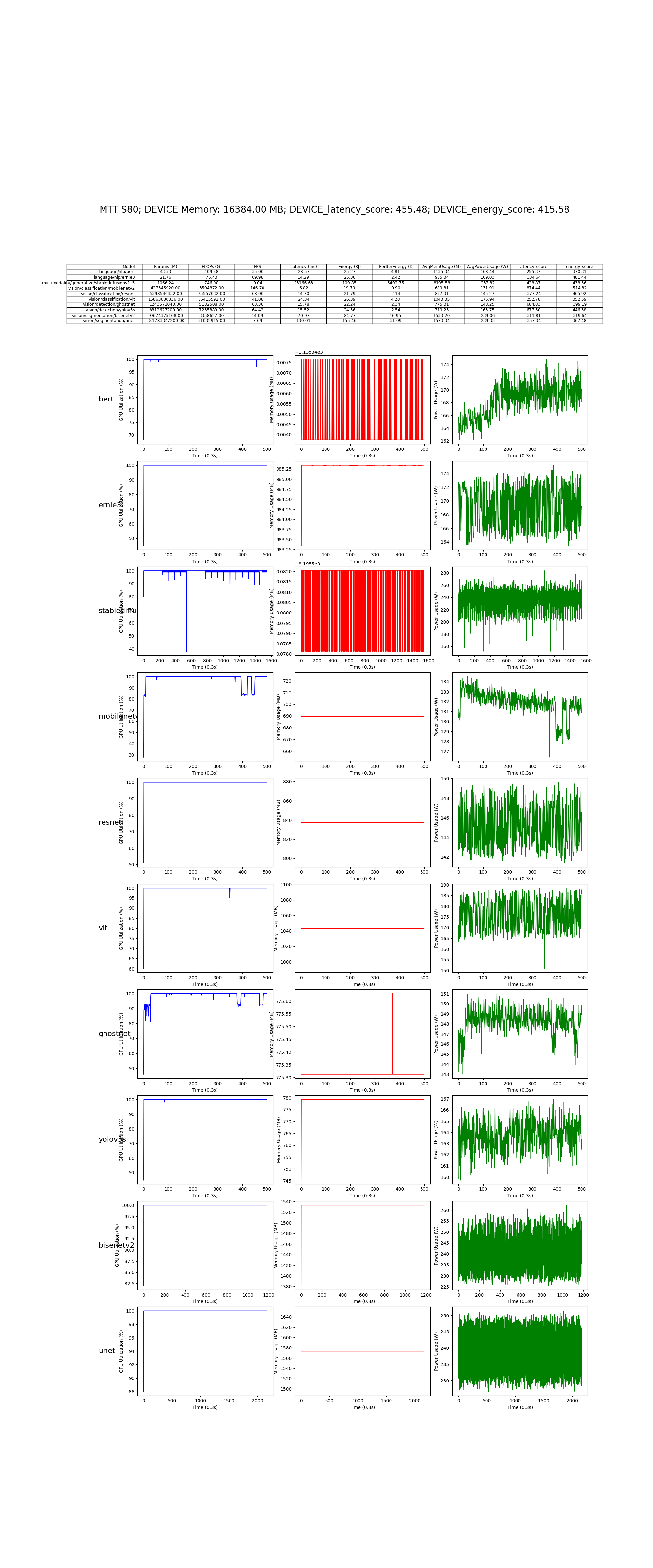
总结与展望
AI架构的技术栈随着硬件平台的多样化和软件生态的不断演进而日益复杂。英伟达凭借其CUDA生态和GPU的强大计算能力,已经成为AI领域的主导者,而AMD则通过其ROCm平台和高性能计算架构逐渐崭露头角,挑战英伟达的垄断地位。与此同时,Intel的AI平台依托其至强处理器与特有的OneAPI框架,在通用计算领域表现突出,具备一定的优势。算能与摩尔线程等国产加速卡也在迅速崛起,成为AI硬件领域的重要力量。依托自主研发的AI芯片,专注于AI推理和训练的高效加速,逐步形成了具有竞争力的解决方案。。未来,AI架构技术栈将朝着更高效的异构计算和跨平台协作方向发展,系统软件与硬件的深度融合将成为优化性能的关键,而技术标准化和开源平台的推广有望进一步推动AI应用的普及与创新。
附录——AI技术栈安装指南
按目录查找即可
NVIDIA平台
CUDA
#!/bin/bash
# 步骤 1: 更新系统并安装必要的依赖
echo "更新系统并安装必要依赖..."
sudo apt-get update
sudo apt-get install -y build-essential dkms
# 步骤 2: 添加 NVIDIA CUDA 工具包存储库
echo "添加 NVIDIA CUDA 存储库..."
wget https://developer.download.nvidia.com/compute/cuda/repos/ubuntu2004/x86_64/cuda-ubuntu2004.pin
sudo mv cuda-ubuntu2004.pin /etc/apt/preferences.d/cuda-repository-pin-600
sudo apt-key adv --fetch-keys https://developer.download.nvidia.com/compute/cuda/repos/ubuntu2004/x86_64/7fa2af80.pub
sudo add-apt-repository "deb https://developer.download.nvidia.com/compute/cuda/repos/ubuntu2004/x86_64/ /"
# 步骤 3: 安装 CUDA 工具包
echo "安装 CUDA 工具包..."
sudo apt-get update
sudo apt-get -y install cuda
# 步骤 4: 设置环境变量
echo "配置 CUDA 环境变量..."
echo 'export PATH=/usr/local/cuda/bin:$PATH' >> ~/.bashrc
echo 'export LD_LIBRARY_PATH=/usr/local/cuda/lib64:$LD_LIBRARY_PATH' >> ~/.bashrc
source ~/.bashrc
# 步骤 5: 验证 CUDA 安装
echo "验证 CUDA 安装..."
nvcc --version
echo "CUDA 安装完成。请重新启动系统以确保更改生效。"
OpenCL (NVIDIA)
#!/bin/bash
# OpenCL ICD安装步骤
echo "开始安装OpenCL ICD..."
# 检查NVIDIA驱动是否已安装
echo "检查NVIDIA驱动安装情况..."
nvidia-smi
# 更新软件包列表
echo "更新软件包列表..."
sudo apt update
# 安装OpenCL ICD和NVIDIA OpenCL开发库
echo "安装OpenCL ICD和NVIDIA OpenCL开发库..."
sudo apt install -y ocl-icd-libopencl1 nvidia-opencl-dev
# 安装clinfo并检查OpenCL安装情况
echo "安装clinfo工具并检查OpenCL平台和设备信息..."
sudo apt-get install -y clinfo
clinfo
# 检查OpenCL头文件是否安装成功
echo "检查OpenCL头文件..."
ls /usr/include/CL
echo "OpenCL ICD安装完成。"
# OpenCL Runtime安装步骤
echo "开始安装OpenCL Runtime..."
# 检查NVIDIA驱动是否已安装
echo "再次检查NVIDIA驱动安装情况..."
nvidia-smi
# 更新软件包列表
echo "更新软件包列表..."
sudo apt update
# 安装CUDA工具包(需要根据操作系统版本替换<distro>和<version>)
echo "安装CUDA工具包..."
CUDA_REPO_PKG="cuda-repo-<distro>_<version>_amd64.deb"
sudo dpkg -i ${CUDA_REPO_PKG}
sudo apt-key adv --fetch-keys https://developer.download.nvidia.com/compute/cuda/repos/<distro>/x86_64/7fa2af80.pub
sudo apt-get update
sudo apt-get install -y cuda
# 配置环境变量
echo "配置CUDA环境变量..."
echo 'export PATH=/usr/local/cuda/bin:$PATH' >> ~/.bashrc
echo 'export LD_LIBRARY_PATH=/usr/local/cuda/lib64:$LD_LIBRARY_PATH' >> ~/.bashrc
source ~/.bashrc
# 安装clinfo并再次检查OpenCL安装情况
echo "再次检查OpenCL平台和设备信息..."
sudo apt-get install -y clinfo
clinfo
echo "OpenCL Runtime安装完成。"
# OpenCL C/C++开发环境安装步骤
echo "开始安装OpenCL C/C++开发环境..."
# 检查NVIDIA驱动是否已安装
echo "检查NVIDIA驱动安装情况..."
nvidia-smi
# 更新软件包列表
echo "更新软件包列表..."
sudo apt update
# 安装CUDA工具包
echo "安装CUDA工具包..."
sudo dpkg -i ${CUDA_REPO_PKG}
sudo apt-key adv --fetch-keys https://developer.download.nvidia.com/compute/cuda/repos/<distro>/x86_64/7fa2af80.pub
sudo apt-get update
sudo apt-get install -y cuda
# 配置环境变量
echo "配置CUDA环境变量..."
echo 'export PATH=/usr/local/cuda/bin:$PATH' >> ~/.bashrc
echo 'export LD_LIBRARY_PATH=/usr/local/cuda/lib64:$LD_LIBRARY_PATH' >> ~/.bashrc
source ~/.bashrc
# 安装OpenCL开发库
echo "安装OpenCL开发库..."
sudo apt-get install -y ocl-icd-opencl-dev
# 测试OpenCL C/C++开发环境(可选:运行C++示例代码)
echo "OpenCL C/C++开发环境安装完成。"
在运行脚本之前,请确保将 <distro> 和 <version> 替换为实际的操作系统版本和CUDA版本。
SYCL(NVIDIA)
#!/bin/bash
# 步骤 1: 安装必要依赖
echo "安装基本依赖..."
sudo apt update
sudo apt install -y cmake pkg-config build-essential
# 验证依赖是否安装成功
echo "验证依赖安装..."
which cmake pkg-config make gcc g++
# 步骤 2: 安装包含DPC++/C++编译器的英特尔oneAPI工具包版本2024.2.1
echo "下载并安装英特尔oneAPI工具包..."
wget https://registrationcenter-download.intel.com/akdlm/IRC_NAS/e6ff8e9c-ee28-47fb-abd7-5c524c983e1c/l_BaseKit_p_2024.2.1.100_offline.sh
sudo sh ./l_BaseKit_p_2024.2.1.100_offline.sh -a --silent --cli --eula accept
# 步骤 3: 安装CUDA(假设已安装,可跳过该步骤)
echo "跳过CUDA安装步骤,假设已安装..."
# 步骤 4: 安装NVIDIA GPU插件
echo "下载并安装NVIDIA GPU插件..."
# 需要自行访问Codeplay下载页面下载插件,根据用户的DPC++/C++版本
wget https://developer.codeplay.com/products/oneapi/nvidia/download/oneapi-for-nvidia-gpus-2024.2.1-cuda-12.0-linux.sh
sudo sh oneapi-for-nvidia-gpus-2024.2.1-cuda-12.0-linux.sh
# 步骤 5: 设置环境变量
echo "设置环境变量..."
# 如果安装为系统范围的安装
echo "设置系统范围的环境变量..."
source /opt/intel/oneapi/setvars.sh --include-intel-llvm
# 如果安装为用户自定义位置,请替换路径为实际的安装路径
# echo "设置私人安装环境变量..."
# source ~/intel/oneapi/setvars.sh --include-intel-llvm
# 确保CUDA库和工具可用
echo "检查CUDA工具和库..."
nvidia-smi
# 如果nvidia-smi出现问题,手动设置CUDA路径
# export PATH=/usr/local/cuda/bin:$PATH
# export LD_LIBRARY_PATH=/usr/local/cuda/lib64:$LD_LIBRARY_PATH
# 步骤 6: 验证安装
echo "验证SYCL安装..."
sycl-ls
# 验证结果
echo "如果输出显示类似以下内容:[cuda:gpu][cuda:0] NVIDIA CUDA BACKEND, NVIDIA A100-PCIE-40GB 8.0 [CUDA 12.5],则安装成功。"
脚本说明:
- 安装必要依赖:更新系统并安装所需的构建工具,如CMake、pkg-config等。
- 安装英特尔oneAPI工具包:下载并以静默方式安装包含DPC++/C++编译器的英特尔oneAPI工具包。
- 安装NVIDIA GPU插件:下载并安装NVIDIA GPU的DPC++插件。
- 设置环境变量:配置英特尔工具链的环境变量,确保正确识别DPC++和CUDA路径。
- 验证安装:通过
sycl-ls命令验证SYCL安装和NVIDIA GPU插件是否成功。
请确保替换脚本中的路径和版本信息以适应您具体的系统环境和安装需求。
计算库
以下是基于您提供的运行SYCL测试例子的自动化脚本。该脚本涵盖了DPC++安装、环境配置、项目克隆和编译的所有步骤。
#!/bin/bash
# 步骤 1: 安装 DPC++(Intel oneAPI)
echo "下载并安装 Intel oneAPI BaseKit..."
wget https://registrationcenter-download.intel.com/akdlm/IRC_NAS/e6ff8e9c-ee28-47fb-abd7-5c524c983e1c/l_BaseKit_p_2024.2.1.100.sh
sudo sh ./l_BaseKit_p_2024.2.1.100.sh -a --silent --cli --eula accept
# 步骤 2: 设置环境变量
echo "设置 Intel oneAPI 环境变量..."
source /opt/intel/oneapi/setvars.sh
# 步骤 3: 配置 CMake 环境
echo "配置 CMake 环境..."
which icpx
export CXX=/opt/intel/oneapi/compiler/2024.2/bin/icpx
# 步骤 4: 克隆 portBLAS 仓库
echo "克隆 portBLAS 仓库..."
git clone https://github.com/codeplaysoftware/portBLAS.git
cd portBLAS
# 步骤 5: 设置临时环境变量
echo "设置临时环境变量..."
SYCL_LIB=$(find / -name libsycl.so.7 2>/dev/null)
export LD_LIBRARY_PATH=/opt/intel/oneapi/2024.2/lib:/opt/intel/oneapi/compiler/2024.2/lib:$LD_LIBRARY_PATH
# 步骤 6: 安装 GCC 11 版本
echo "安装 GCC 11 和相关依赖库..."
sudo apt install -y gcc-11 g++-11
# 步骤 7: 安装 OpenMP 和 OpenBLAS
echo "安装 OpenMP 和 OpenBLAS..."
sudo apt-get install -y libomp-dev libopenblas-dev
# 步骤 8: 编译 portBLAS
echo "开始编译 portBLAS..."
mkdir -p build && cd build
cmake -GNinja ../ -DSYCL_COMPILER=dpcpp -DDPCPP_SYCL_TARGET=nvptx64-nvidia-cuda -DDPCPP_SYCL_ARCH=sm_80 -DCMAKE_INSTALL_PREFIX=/usr/local/portBLAS
# 使用 Ninja 进行构建和安装
ninja
sudo ninja install
# 步骤 9: 运行示例程序
echo "运行 sample_gemm 示例程序..."
./samples/sample_gemm
# 如果遇到 CMake 配置错误,清理缓存后重新配置
if [ $? -ne 0 ]; then
echo "CMake 配置失败,清理缓存并重新配置..."
rm -rf CMakeCache.txt CMakeFiles
cmake -GNinja ../ -DSYCL_COMPILER=dpcpp -DDPCPP_SYCL_TARGET=nvptx64-nvidia-cuda -DDPCPP_SYCL_ARCH=sm_80 -DCMAKE_INSTALL_PREFIX=/usr/local/portBLAS
ninja
sudo ninja install
fi
# 步骤 10: 编译自定义算子
echo "编译自定义 SYCL 代码..."
icpx -fsycl -o test_device ../samples/test.cpp
./test_device
echo "SYCL 测试完成。"
脚本说明:
- 安装Intel oneAPI:下载并以静默方式安装Intel oneAPI BaseKit。
- 设置环境变量:配置SYCL编译器的环境变量,确保DPC++正确使用。
- 克隆portBLAS仓库:从GitHub克隆portBLAS代码库。
- 配置CMake和编译选项:通过CMake进行配置,指定使用NVIDIA GPU并使用Ninja构建工具编译。
- 运行示例:编译并运行
sample_gemm示例测试SYCL环境。 - 编译自定义SYCL代码:编译并运行自定义的SYCL程序
test_device。
Triton (NVIDIA)
#!/bin/bash
# 步骤 1: 更新系统
echo "更新系统..."
sudo apt-get update && sudo apt-get upgrade -y
# 步骤 2: 检查 CUDA 是否安装
echo "检查 CUDA 安装情况..."
if ! command -v nvcc &> /dev/null
then
echo "CUDA 未安装,请先安装 CUDA。"
exit 1
else
nvcc --version
fi
# 步骤 3: 检查 NVIDIA 驱动是否安装
echo "检查 NVIDIA 驱动安装情况..."
if ! command -v nvidia-smi &> /dev/null
then
echo "NVIDIA 驱动未安装,请先安装驱动。"
exit 1
else
nvidia-smi
fi
# 步骤 4: 安装 Python 3.9 和 pip
echo "安装 Python 3.9 和 pip..."
sudo apt-get install -y python3 python3-pip
# 步骤 5: 安装 PyTorch (CUDA 11.8 版本)
echo "安装 PyTorch..."
pip install torch torchvision torchaudio --index-url https://download.pytorch.org/whl/cu118
# 步骤 6: 安装 Triton
echo "安装 Triton..."
pip install triton
# 验证 Triton 安装
echo "验证 Triton 安装..."
python3 -c "import triton; print(triton.__version__)"
echo "Triton 安装完成。"
脚本说明:
- 系统更新:首先更新系统软件包并升级现有软件。
- 检查CUDA和驱动:检查系统是否已安装CUDA和NVIDIA驱动,如果未安装则终止脚本执行。
- 安装Python 3.9:通过APT安装Python 3.9及其对应的pip工具。
- 安装PyTorch:通过
pip安装支持CUDA 11.8的PyTorch及相关库。 - 安装Triton:通过
pip安装Triton库。 - 验证Triton安装:通过Python命令检查Triton版本以确保安装成功。
此脚本将自动执行所有步骤,确保环境配置正确并安装Triton。
Apache TVM (NVIDIA)
#!/bin/bash
# 步骤 1: 安装依赖项
echo "更新系统并安装依赖项..."
sudo apt-get update
sudo apt-get install -y git cmake build-essential libtinfo-dev zlib1g-dev \
libcurl4-openssl-dev libopenblas-dev python3-dev \
python3-pip python3-setuptools python3-venv
# 步骤 2: 克隆 Apache TVM 的 GitHub 仓库
echo "克隆 Apache TVM 的 GitHub 仓库..."
git clone --recursive https://github.com/apache/tvm.git
cd tvm
# 步骤 3: 安装 LLVM
echo "安装 LLVM..."
sudo apt-get install -y llvm llvm-dev clang
# 步骤 4: 配置 TVM
echo "配置 TVM..."
mkdir build
cd build
cmake .. -DUSE_CUDA=ON -DUSE_CUDNN=ON -DUSE_LLVM=ON -DCMAKE_BUILD_TYPE=Release
# 步骤 5: 构建 TVM
echo "构建 TVM..."
make -j$(nproc)
# 步骤 6: 设置环境变量
echo "设置 TVM 环境变量..."
echo 'export TVM_HOME=~/tvm' >> ~/.bashrc
echo 'export PYTHONPATH=$TVM_HOME/python:${PYTHONPATH}' >> ~/.bashrc
echo 'export PATH=$TVM_HOME/build:${PATH}' >> ~/.bashrc
source ~/.bashrc
# 步骤 7: 安装 Python 依赖项
echo "安装 Python 依赖项..."
pip install numpy
pip install -e ${TVM_HOME}/python
# 步骤 8: 验证安装并解决可能的 libstdc++.so.6 问题
echo "验证 TVM 安装..."
python3 -c "import tvm; print('TVM version:', tvm.__version__)"
# 如果缺少 .so 文件,运行以下步骤
echo "检查并处理 libstdc++.so.6 相关问题..."
ldd $(which python3) | grep libstdc++
if [ $? -ne 0 ]; then
echo "设置 LD_PRELOAD 以解决 libstdc++.so.6 问题..."
export LD_PRELOAD=/usr/lib/x86_64-linux-gnu/libstdc++.so.6
fi
echo "Apache TVM 安装完成。"
脚本说明:
- 安装依赖项:首先更新系统并安装构建TVM所需的依赖项,包括CMake、LLVM、Python开发工具等。
- 克隆TVM仓库:从Apache TVM官方GitHub仓库克隆源代码。
- 安装LLVM:安装LLVM相关工具,用于支持TVM的编译。
- 配置和构建TVM:启用CUDA、CUDNN和LLVM支持,使用CMake配置和构建TVM。
- 设置环境变量:将TVM路径添加到系统的
PYTHONPATH和PATH中,以确保能够正确加载TVM库。 - 安装Python依赖项:安装TVM所需的Python依赖,包括
numpy等。 - 验证安装:通过Python测试TVM是否安装成功,并检查是否存在
libstdc++.so.6版本问题。
运行此脚本将自动完成Apache TVM的安装及环境配置,并验证是否正确安装。
OpenXLA (NVIDIA)
#!/bin/bash
# 步骤 1: 更新系统并安装基本依赖
echo "更新系统并安装必要依赖..."
sudo apt-get update
sudo apt-get install -y build-essential git cmake python3 python3-pip python3-venv
# 步骤 2: 克隆 OpenXLA 项目
echo "克隆 OpenXLA 项目..."
git clone https://github.com/openxla/openxla.git
cd openxla
# 步骤 3: 创建 Python 虚拟环境
echo "创建 Python 虚拟环境..."
python3 -m venv venv
source venv/bin/activate
# 步骤 4: 安装 OpenXLA 依赖
echo "安装 OpenXLA 依赖..."
pip install --upgrade pip
pip install -r requirements.txt
# 步骤 5: 安装 Bazel(用于编译 OpenXLA)
echo "安装 Bazel..."
sudo apt-get install apt-transport-https curl gnupg -y
curl -fsSL https://bazel.build/bazel-release.pub.gpg | gpg --dearmor >bazel-archive-keyring.gpg
sudo mv bazel-archive-keyring.gpg /usr/share/keyrings/bazel-archive-keyring.gpg
echo "deb [signed-by=/usr/share/keyrings/bazel-archive-keyring.gpg] https://storage.googleapis.com/bazel-apt stable jdk1.8" | sudo tee /etc/apt/sources.list.d/bazel.list
sudo apt-get update && sudo apt-get install bazel
# 步骤 6: 编译 OpenXLA
echo "编译 OpenXLA..."
bazel build ...
# 步骤 7: 配置 CUDA 和 cuDNN(假设 CUDA 和 cuDNN 已安装)
echo "配置 CUDA 和 cuDNN 环境变量..."
echo 'export PATH=/usr/local/cuda/bin:$PATH' >> ~/.bashrc
echo 'export LD_LIBRARY_PATH=/usr/local/cuda/lib64:$LD_LIBRARY_PATH' >> ~/.bashrc
source ~/.bashrc
# 步骤 8: 验证安装
echo "验证 OpenXLA 安装..."
python -c "import openxla; print('OpenXLA 安装成功!')"
echo "OpenXLA 安装完成!"
脚本说明:
- 更新系统和安装依赖:安装构建OpenXLA所需的基本工具,包括
git、cmake、python3、pip等。 - 克隆OpenXLA项目:从GitHub克隆OpenXLA源代码。
- 创建Python虚拟环境:使用
python3-venv创建Python虚拟环境并激活它,以隔离依赖项。 - 安装依赖:通过
pip安装OpenXLA项目所需的依赖。 - 安装Bazel:Bazel是一个用于构建和测试项目的构建工具,OpenXLA的构建依赖于Bazel。
- 编译OpenXLA:使用Bazel编译OpenXLA源代码。
- 配置CUDA和cuDNN:假设已经安装了CUDA和cuDNN,设置环境变量以确保它们可以被OpenXLA使用。
- 验证安装:通过Python导入OpenXLA模块,确保安装成功。
OpenACC
#!/bin/bash
# 步骤 1: 下载并解压安装 NVIDIA HPC SDK
echo "下载并安装 NVIDIA HPC SDK..."
wget https://developer.download.nvidia.com/hpc-sdk/24.7/nvhpc_2024_247_Linux_x86_64_cuda_multi.tar.gz
tar xpzf nvhpc_2024_247_Linux_x86_64_cuda_multi.tar.gz
cd nvhpc_2024_247_Linux_x86_64_cuda_multi
sudo ./install
# 步骤 2: 设置环境变量
echo "设置环境变量..."
echo 'export PATH=/opt/nvidia/hpc_sdk/Linux_x86_64/24.7/compilers/bin:$PATH' >> ~/.bashrc
echo 'export LD_LIBRARY_PATH=/opt/nvidia/hpc_sdk/Linux_x86_64/24.7/compilers/lib:$LD_LIBRARY_PATH' >> ~/.bashrc
source ~/.bashrc
# 步骤 3: 创建测试代码
echo "创建测试代码 matrix_add.c..."
cat <<EOL > matrix_add.c
#include <stdio.h>
#include <stdlib.h>
#include <time.h>
#include <openacc.h>
#define N 10000
void matrix_add_cpu(float *A, float *B, float *C, int n) {
for (int i = 0; i < n; i++) {
for (int j = 0; j < n; j++) {
C[i * n + j] = A[i * n + j] + B[i * n + j];
}
}
}
void matrix_add_gpu(float *A, float *B, float *C, int n) {
#pragma acc parallel loop collapse(2) copyin(A[0:n*n], B[0:n*n]) copyout(C[0:n*n])
for (int i = 0; i < n; i++) {
for (int j = 0; j < n; j++) {
C[i * n + j] = A[i * n + j] + B[i * n + j];
}
}
}
int main() {
float *A, *B, *C;
A = (float*) malloc(N * N * sizeof(float));
B = (float*) malloc(N * N * sizeof(float));
C = (float*) malloc(N * N * sizeof(float));
srand(time(0));
for (int i = 0; i < N * N; i++) {
A[i] = (float)rand() / RAND_MAX;
B[i] = (float)rand() / RAND_MAX;
}
clock_t start_cpu = clock();
matrix_add_cpu(A, B, C, N);
clock_t end_cpu = clock();
double cpu_time = (double)(end_cpu - start_cpu) / CLOCKS_PER_SEC;
printf("CPU Time: %f seconds\\n", cpu_time);
clock_t start_gpu = clock();
matrix_add_gpu(A, B, C, N);
clock_t end_gpu = clock();
double gpu_time = (double)(end_gpu - start_gpu) / CLOCKS_PER_SEC;
printf("GPU Time: %f seconds\\n", gpu_time);
free(A);
free(B);
free(C);
return 0;
}
EOL
# 步骤 4: 编译并运行测试程序
echo "编译并运行测试程序..."
pgcc -acc -Minfo=accel -o matrix_add matrix_add.c
./matrix_add
脚本说明:
- 下载并安装NVIDIA HPC SDK:该脚本会从NVIDIA官网下载最新的HPC SDK(24.7版本),解压并进行安装。
- 设置环境变量:将HPC SDK的编译器路径和库路径添加到系统的
PATH和LD_LIBRARY_PATH中,并立即生效。 - 创建测试代码:生成一个
matrix_add.c的OpenACC测试代码,其中包含矩阵加法的CPU和GPU实现。 - 编译并运行测试代码:使用
pgcc编译器编译该OpenACC代码,并输出运行时间来对比CPU和GPU的执行时间。
AMD 平台
ROCm / HIP
#!/bin/bash
# 步骤 1: 添加 ROCm 存储库
echo "添加 ROCm 存储库..."
# 添加 GPG 密钥
wget -qO - http://repo.radeon.com/rocm/rocm.gpg.key | sudo apt-key add -
# 添加存储库地址到 sources.list.d
echo 'deb [arch=amd64] http://repo.radeon.com/rocm/apt/5.7/ ubuntu main' | sudo tee /etc/apt/sources.list.d/rocm.list
# 步骤 2: 更新 APT 包缓存
echo "更新 APT 包缓存..."
sudo apt update
# 步骤 3: 安装 ROCm 软件包
echo "安装 ROCm 堆栈..."
sudo apt install -y rocm-dkms
# 步骤 4: 设置环境变量
echo "设置 ROCm 环境变量..."
echo 'export PATH=$PATH:/opt/rocm/bin' >> ~/.bashrc
echo 'export LD_LIBRARY_PATH=$LD_LIBRARY_PATH:/opt/rocm/lib' >> ~/.bashrc
# 使环境变量生效
echo "应用环境变量..."
source ~/.bashrc
# 步骤 5: 验证安装
echo "验证 ROCm 安装..."
/opt/rocm/bin/rocminfo
# 步骤 6: 安装 HIP 编程环境
echo "安装 HIP 基础工具..."
sudo apt install -y hip-base
# 步骤 7: 验证编译示例程序
echo "克隆并编译 HIP 示例程序..."
git clone https://github.com/ROCm-Developer-Tools/HIP-Examples.git
cd HIP-Examples/vectorAdd
make
# 验证成功运行
echo "运行 vectorAdd 示例程序..."
./vectorAdd
echo "ROCm 和 HIP 安装及测试完成。"
脚本说明:
- 添加ROCm存储库:从AMD官方源下载GPG密钥并添加软件包存储库。
- 更新APT包缓存:更新系统的包缓存。
- 安装ROCm堆栈:通过APT安装整个ROCm堆栈,包含核心驱动、工具和库。
- 设置环境变量:将ROCm路径添加到环境变量
PATH和LD_LIBRARY_PATH中,并立即生效。 - 验证安装:使用
rocminfo命令验证ROCm是否正确安装。 - 安装HIP编程环境:安装HIP的基本工具和SDK。
- 编译并运行HIP示例程序:克隆AMD提供的HIP示例代码库,编译并运行
vectorAdd示例,验证HIP编程环境是否成功搭建。
该脚本会自动执行所有步骤,确保ROCm和HIP在AMD平台上的正确安装和配置。
算子库
以下是您提供的ROCm相关算子库的编译过程总结的自动化脚本,涵盖了hipBLAS-common、hipBLASLt、rocBLAS等库的安装和自定义编译步骤。
#!/bin/bash
# 步骤 1: 克隆并编译 hipBLAS-common
echo "克隆并编译 hipBLAS-common..."
git clone https://github.com/ROCm/hipBLAS-common.git
cd hipBLAS-common
mkdir build && cd build
cmake ..
make package install
cd ../..
# 步骤 2: 安装 hipBLASLt
echo "安装 hipBLASLt 开发包..."
sudo apt-get install -y hipblas-dev hipblaslt-dev
# 运行 hipBLASLt 安装脚本
echo "运行 hipBLASLt 安装脚本..."
git clone https://github.com/ROCm/hipBLASLt.git
cd hipBLASLt
./install.sh -idc --legacy_hipblas_direct --architecture 'gfx1100'
cd ..
# 步骤 3: 安装 rocBLAS 并自定义编译
echo "安装 rocBLAS..."
git clone https://github.com/ROCm/rocBLAS.git
cd rocBLAS
./install.sh -idc
# 自定义编译 rocBLAS 测试程序
echo "自定义编译 rocBLAS 测试程序..."
sudo hipcc -o rocblas_test clients/samples/rocblas_test.cpp -lrocblas
cd ..
# 步骤 4: 编译 hipBLAS 测试程序
echo "编译 hipBLAS 测试程序..."
sudo hipcc -o hipblas_test hipBLAS-common/clients/samples/hipblas_test.cpp -I/opt/rocm/include/hipblas -lhipblas
# 步骤 5: 设置 ROCm 环境变量
echo "设置 ROCm 环境变量..."
export HIP_PATH=/opt/rocm
export PATH=$PATH:$HIP_PATH/bin
export LD_LIBRARY_PATH=$LD_LIBRARY_PATH:$HIP_PATH/lib
echo "ROCm 算子库编译完成。"
脚本说明:
- hipBLAS-common:克隆并编译
hipBLAS-common库,创建build目录,使用CMake进行配置和编译。 - hipBLASLt:安装
hipBLAS和hipBLASLt开发包,运行hipBLASLt的安装脚本,并指定相关架构。 - rocBLAS:克隆并安装
rocBLAS,并编译自定义的rocblas_test测试程序。 - hipBLAS测试:使用
hipcc编译hipBLAS的测试程序,并包含必要的头文件和库。 - 设置环境变量:将
HIP_PATH和LD_LIBRARY_PATH设置为ROCm的安装路径,确保运行时可以找到必要的工具和库。
此脚本将自动执行ROCm相关算子库的安装和编译步骤,确保环境正确配置和可执行程序生成。
OpenCL (AMD)
#!/bin/bash
# 更新系统软件包
echo "更新系统软件包..."
sudo apt update && sudo apt upgrade -y
# 添加 ROCm 官方软件源
echo "添加 ROCm 官方软件源..."
wget -qO - http://repo.radeon.com/rocm/rocm.gpg.key | sudo apt-key add -
echo 'deb [arch=amd64] http://repo.radeon.com/rocm/apt/debian/ xenial main' | sudo tee /etc/apt/sources.list.d/rocm.list
# 更新软件包索引
echo "更新软件包索引..."
sudo apt update
# 安装 ROCm 和 OpenCL Runtime
echo "安装 ROCm 和 OpenCL Runtime..."
sudo apt install -y rocm-dkms rocm-opencl rocm-opencl-dev
# 设置环境变量
echo "设置环境变量..."
echo 'export PATH=/opt/rocm/bin:$PATH' >> ~/.bashrc
echo 'export LD_LIBRARY_PATH=/opt/rocm/lib:$LD_LIBRARY_PATH' >> ~/.bashrc
# 使环境变量生效
echo "应用环境变量..."
source ~/.bashrc
# 验证 OpenCL 安装
echo "验证 OpenCL 安装..."
clinfo
# 安装必要的依赖库(可选)
echo "安装必要的依赖库..."
sudo apt install -y ocl-icd-libopencl1 opencl-headers clinfo
echo "OpenCL 安装完成。"
脚本说明:
- 脚本会首先更新系统的软件包,然后添加ROCm仓库。
- 安装ROCm驱动和OpenCL Runtime。
- 自动将环境变量添加到
~/.bashrc文件,并立即生效。 - 通过
clinfo验证OpenCL安装是否成功。 - 可选步骤是安装一些OpenCL开发所需的依赖库。
运行该脚本前,建议先确保操作系统版本支持ROCm,并根据需求修改部分配置。
SYCL (AMD)
#!/bin/bash
# 步骤 1: 安装必要依赖
echo "安装必要依赖..."
sudo apt -y install cmake pkg-config build-essential
# 步骤 2: 下载并安装英特尔 oneAPI 工具包
echo "下载并安装 Intel oneAPI BaseKit..."
wget https://registrationcenter-download.intel.com/akdlm/IRC_NAS/e6ff8e9c-ee28-47fb-abd7-5c524c983e1c/l_BaseKit_p_2024.2.1.100_offline.sh
sudo sh ./l_BaseKit_p_2024.2.1.100_offline.sh -a --silent --cli --eula accept
# 步骤 3: 下载并安装 AMD 对应 DPC++/C++ 插件
echo "下载并安装 AMD 对应的 DPC++/C++ 插件..."
wget https://developer.codeplay.com/products/oneapi/amd/download/oneapi-for-amd-gpus-2024.2.1-rocm-5.4.3-linux.sh
sudo sh oneapi-for-amd-gpus-2024.2.1-rocm-5.4.3-linux.sh
# 步骤 4: 设置环境变量
echo "设置 oneAPI 环境变量..."
source /opt/intel/oneapi/setvars.sh --include-intel-llvm
# 步骤 5: 验证 SYCL 安装
echo "验证 SYCL 安装..."
sycl-ls
# 步骤 6: 创建 SYCL 示例程序
echo "创建 SYCL 示例程序..."
cat <<EOL > simple-sycl-app.cpp
#include <sycl/sycl.hpp>
int main() {
sycl::buffer<int, 1> Buffer{4};
sycl::queue Queue{};
sycl::range<1> NumOfWorkItems{Buffer.size()};
Queue.submit([&](sycl::handler &cgh) {
auto Accessor = Buffer.get_access<sycl::access::mode::write>(cgh);
cgh.parallel_for<class FillBuffer>(
NumOfWorkItems, [=](sycl::id<1> WIid) {
Accessor[WIid] = static_cast<int>(WIid.get(0));
});
});
auto HostAccessor = Buffer.get_host_access();
bool MismatchFound{false};
for (size_t I{0}; I < Buffer.size(); ++I) {
if (HostAccessor[I] != I) {
std::cout << "The result is incorrect for element: " << I
<< " , expected: " << I << " , got: " << HostAccessor[I]
<< std::endl;
MismatchFound = true;
}
}
if (!MismatchFound) {
std::cout << "The results are correct!" << std::endl;
}
return MismatchFound;
}
EOL
# 步骤 7: 获取 AMD GPU 的架构名称
echo "获取 AMD GPU 架构信息..."
ARCH=$(rocminfo | grep 'Name: *gfx' | awk '{print $2}')
# 步骤 8: 编译 SYCL 示例程序
echo "编译 SYCL 示例程序..."
icpx -fsycl -fsycl-targets=amdgcn-amd-amdhsa -Xsycl-target-backend --offload-arch=$ARCH -o simple-sycl-app simple-sycl-app.cpp
# 步骤 9: 运行 SYCL 示例程序
echo "运行 SYCL 示例程序..."
ONEAPI_DEVICE_SELECTOR="hip:*" SYCL_PI_TRACE=1 ./simple-sycl-app
echo "SYCL 安装和示例运行完成。"
脚本说明:
- 安装依赖:首先安装构建SYCL程序所需的基本工具如CMake、pkg-config等。
- 下载并安装Intel oneAPI工具包:下载并安装Intel提供的oneAPI BaseKit,用于支持DPC++编译器和SYCL环境。
- 安装AMD对应的DPC++插件:从Codeplay官网下载并安装针对AMD GPU的DPC++插件,确保AMD GPU可以使用SYCL编译和运行。
- 设置环境变量:使用Intel提供的
setvars.sh脚本配置环境变量,确保工具链和库正确配置。 - 验证SYCL安装:通过
sycl-ls命令验证SYCL平台和设备是否正确安装。 - 创建并编译SYCL程序:编写一个简单的SYCL程序来测试平台配置,并使用
icpx编译该程序,针对AMD GPU架构生成代码。 - 运行SYCL程序:设置环境变量
ONEAPI_DEVICE_SELECTOR为hip:*以选择AMD GPU,并运行编译好的程序进行测试。
该脚本将自动执行所有步骤,确保SYCL在AMD平台上的正确安装和运行,并且提供了一个简单的示例以验证环境配置。
Triton (AMD)
#!/bin/bash
# 步骤 1: 安装必要依赖
echo "更新系统软件包并安装必要依赖..."
sudo apt update
sudo apt install -y python3 python3-pip clang
# 步骤 2: 添加 ROCm 软件源并安装 ROCm
echo "添加 ROCm 软件源..."
wget -qO - http://repo.radeon.com/rocm/rocm.gpg.key | sudo apt-key add -
echo 'deb [arch=amd64] http://repo.radeon.com/rocm/apt/debian/ xenial main' | sudo tee /etc/apt/sources.list.d/rocm.list
# 更新软件包列表并安装 ROCm
echo "更新软件包列表并安装 ROCm..."
sudo apt update
sudo apt install -y rocm-dkms rocm-dev rocm-opencl
# 设置环境变量
echo "设置 ROCm 环境变量..."
echo 'export PATH=/opt/rocm/bin:$PATH' >> ~/.bashrc
echo 'export LD_LIBRARY_PATH=/opt/rocm/lib:$LD_LIBRARY_PATH' >> ~/.bashrc
source ~/.bashrc
# 步骤 3: 安装 Triton 和相关依赖
echo "安装 Triton 和 pybind11..."
pip install pybind11==2.13.1
pip install triton
echo "Triton 安装完成。"
脚本说明:
- 脚本会先安装Python、Pip和Clang作为必要依赖。
- 添加ROCm的官方软件源,安装所需的ROCm库和驱动程序。
- 设置环境变量以确保系统正确识别ROCm。
- 最后通过
pip安装pybind11和triton库。
运行该脚本时,请确保系统兼容ROCm,另外需要根据具体需求进行微调。
Apache TVM (AMD)
#!/bin/bash
# 步骤 1: 安装基本依赖
echo "安装基本依赖..."
sudo apt update
sudo apt install -y git cmake build-essential libtinfo-dev zlib1g-dev \
python3-dev python3-setuptools python3-pip
# 步骤 2: 安装 LLVM
echo "安装 LLVM..."
sudo apt install -y llvm clang
# 步骤 3: 克隆 Apache TVM 源码
echo "克隆 Apache TVM 源码..."
git clone --recursive https://github.com/apache/tvm tvm
cd tvm
# 步骤 4: 安装 ROCm(适用于 AMD 显卡)
echo "添加 ROCm 仓库并安装 ROCm..."
sudo apt update
sudo apt install -y wget gnupg2
wget -qO - http://repo.radeon.com/rocm/rocm.gpg.key | sudo apt-key add -
echo 'deb [arch=amd64] http://repo.radeon.com/rocm/apt/5.5 ubuntu main' | sudo tee /etc/apt/sources.list.d/rocm.list
# 安装 ROCm
sudo apt update
sudo apt install -y rocm-dkms
# 步骤 5: 编译 Apache TVM
echo "开始编译 Apache TVM..."
cp cmake/config.cmake .
# 配置使用 LLVM 和 ROCm
sed -i '/set(USE_LLVM OFF)/c\set(USE_LLVM llvm-config)' cmake/config.cmake
sed -i '/set(USE_ROCM OFF)/c\set(USE_ROCM ON)' cmake/config.cmake
# 创建构建目录并编译
mkdir build
cd build
cmake ..
make -j$(nproc)
# 步骤 6: 设置 Python 环境
echo "设置 Python 环境..."
cd ../python
sudo python3 setup.py install
# 步骤 7: 验证安装
echo "验证 TVM 安装..."
python3 -c "import tvm; print('TVM 安装成功')"
echo "Apache TVM 安装完成。"
脚本说明:
- 安装基本依赖:首先安装构建TVM所需的基本工具,如Git、CMake和Python开发库。
- 安装LLVM:TVM依赖LLVM进行编译和优化。
- 克隆TVM源码:克隆官方Apache TVM的源码。
- 安装ROCm:适用于AMD显卡的支持,添加ROCm仓库并安装驱动。
- 编译TVM:将
USE_LLVM设置为llvm-config,启用USE_ROCM支持,并编译TVM。 - 设置Python环境:安装Python相关的TVM库,确保TVM可以通过Python调用。
- 验证安装:通过导入
tvm模块验证TVM是否正确安装。
运行该脚本时,请根据系统兼容性确保步骤配置正确,特别是ROCm部分。
OpenXLA (AMD)
以下是一个在AMD平台上安装OpenXLA的自动化脚本。该脚本假设您已经安装了ROCm(用于AMD GPU的并行计算平台),并配置好了ROCm相关的库和工具。
#!/bin/bash
# 步骤 1: 更新系统并安装基本依赖
echo "更新系统并安装必要依赖..."
sudo apt-get update
sudo apt-get install -y build-essential git cmake python3 python3-pip python3-venv
# 步骤 2: 安装 ROCm (如果还未安装)
# 注意:此步骤假设您使用的是 Ubuntu 20.04/22.04
echo "安装 ROCm..."
wget -qO - http://repo.radeon.com/rocm/rocm.gpg.key | sudo apt-key add -
echo 'deb [arch=amd64] http://repo.radeon.com/rocm/apt/5.5/ ubuntu main' | sudo tee /etc/apt/sources.list.d/rocm.list
sudo apt update
sudo apt install -y rocm-dkms rocm-dev rocm-libs hipcub rocprim
# 步骤 3: 设置 ROCm 环境变量
echo "设置 ROCm 环境变量..."
echo 'export PATH=/opt/rocm/bin:$PATH' >> ~/.bashrc
echo 'export LD_LIBRARY_PATH=/opt/rocm/lib:$LD_LIBRARY_PATH' >> ~/.bashrc
source ~/.bashrc
# 步骤 4: 验证 ROCm 安装
echo "验证 ROCm 安装..."
/opt/rocm/bin/rocminfo
/opt/rocm/opencl/bin/x86_64/clinfo
# 步骤 5: 克隆 OpenXLA 项目
echo "克隆 OpenXLA 项目..."
git clone https://github.com/openxla/openxla.git
cd openxla
# 步骤 6: 创建 Python 虚拟环境
echo "创建 Python 虚拟环境..."
python3 -m venv venv
source venv/bin/activate
# 步骤 7: 安装 OpenXLA 依赖
echo "安装 OpenXLA 依赖..."
pip install --upgrade pip
pip install -r requirements.txt
# 步骤 8: 安装 Bazel (用于构建 OpenXLA)
echo "安装 Bazel..."
sudo apt install apt-transport-https curl gnupg -y
curl -fsSL https://bazel.build/bazel-release.pub.gpg | gpg --dearmor >bazel-archive-keyring.gpg
sudo mv bazel-archive-keyring.gpg /usr/share/keyrings/bazel-archive-keyring.gpg
echo "deb [signed-by=/usr/share/keyrings/bazel-archive-keyring.gpg] https://storage.googleapis.com/bazel-apt stable jdk1.8" | sudo tee /etc/apt/sources.list.d/bazel.list
sudo apt-get update && sudo apt-get install bazel
# 步骤 9: 编译 OpenXLA
echo "编译 OpenXLA..."
bazel build ...
# 步骤 10: 验证 OpenXLA 安装
echo "验证 OpenXLA 安装..."
python -c "import openxla; print('OpenXLA 安装成功!')"
echo "OpenXLA 安装完成!"
脚本说明:
- 安装依赖:首先更新系统,并安装必要的依赖,包括构建工具和Python包管理工具。
- 安装ROCm:如果ROCm未安装,使用这个步骤来安装ROCm,包括
rocm-dkms、rocm-dev等基本工具。ROCm是AMD平台上的并行计算框架,类似于NVIDIA的CUDA。 - 设置ROCm环境变量:配置系统的环境变量,确保ROCm工具可以在终端中正确使用。
- 验证ROCm安装:通过运行
rocminfo和clinfo验证ROCm是否正确安装。 - 克隆OpenXLA项目:从GitHub克隆OpenXLA的源代码。
- 创建Python虚拟环境:使用Python虚拟环境隔离依赖,确保项目运行环境独立。
- 安装OpenXLA依赖:通过
pip安装OpenXLA所需的Python依赖项。 - 安装Bazel:Bazel是OpenXLA的构建工具,这一步骤安装Bazel,确保可以正确编译OpenXLA。
- 编译OpenXLA:使用Bazel编译OpenXLA源代码。
- 验证OpenXLA安装:通过Python导入OpenXLA模块,检查是否安装成功。
ONNX (AMD)
#!/bin/bash
# 步骤 1: 验证是否已安装 Radeon Software for Linux (包含 ROCm)
echo "检查是否已安装 ROCm..."
if ! dpkg -l | grep -i rocm; then
echo "未检测到 ROCm,确保您已成功安装 Radeon Software for Linux (带有 ROCm)。"
exit 1
else
echo "ROCm 已安装。"
fi
# 步骤 2: 验证是否已安装 MIGraphX
echo "检查 MIGraphX 安装情况..."
dpkg -l | grep migraphx
if [ $? -ne 0 ]; then
echo "MIGraphX 未安装,请先安装 MIGraphX。"
exit 1
else
echo "MIGraphX 已安装。"
fi
# 验证是否已安装 half 库
echo "检查 half 库安装情况..."
dpkg -l | grep half
if [ $? -ne 0 ]; then
echo "half 库未安装,正在安装 half 库..."
sudo apt install half -y
else
echo "half 库已安装。"
fi
# 步骤 3: 使用 PIP 安装 ONNX Runtime
echo "卸载现有的 onnxruntime-rocm 和 numpy..."
pip3 uninstall onnxruntime-rocm numpy -y
echo "安装 ONNX Runtime 和 numpy..."
pip3 install https://repo.radeon.com/rocm/manylinux/rocm-rel-6.1.3/onnxruntime_rocm-1.17.0-cp310-cp310-linux_x86_64.whl numpy==1.26.4
# 步骤 4: 验证 ONNX Runtime 安装
echo "验证 ONNX Runtime 安装..."
python3 -c "
import onnxruntime as ort
providers = ort.get_available_providers()
print('可用的执行提供者:', providers)
if 'MIGraphXExecutionProvider' in providers and 'ROCMExecutionProvider' in providers and 'CPUExecutionProvider' in providers:
print('ONNX Runtime 安装成功!')
else:
print('ONNX Runtime 安装失败,请检查日志。')
"
echo "ONNX Runtime 安装完成。"
脚本说明:
- 验证ROCm和MIGraphX安装:首先检查是否安装了Radeon Software for Linux和MIGraphX。如果没有安装MIGraphX,则会提示错误。
- 验证
half库安装:检查是否已安装half库,如果未安装,则自动安装它。 - 安装ONNX Runtime:通过PIP安装预构建的ONNX Runtime wheel文件,并将
numpy降级到兼容的版本1.26.4。 - 验证ONNX Runtime安装:通过Python脚本检查ONNX Runtime的可用执行提供者(Execution Providers),确认MIGraphX、ROCM和CPU执行提供者是否可用。
运行此脚本将自动完成AMD平台上ONNX Runtime的安装和配置。
Intel 平台
oneAPI
#!/bin/bash
# 步骤 1: 为 OpenGL 和 Vulkan 配置开源 Mesa 3D 图形库
echo "配置 OpenGL 和 Vulkan 的 Mesa 3D 图形库..."
sudo add-apt-repository ppa:oibaf/graphics-drivers
sudo apt update
sudo apt upgrade -y
# 验证 Mesa 安装
dpkg -l | grep -i mesa
# 步骤 2: 设置环境变量以使用独立显卡
echo "设置环境变量..."
export DRI_PRIME=1
glxinfo -B | grep -i device
glmark2
# 步骤 3: 下载并安装 Intel GPU 必需的软件包
echo "下载并安装 Intel GPU 必需的软件包..."
mkdir -p neo && cd neo
wget https://github.com/intel/intel-graphics-compiler/releases/download/igc-1.0.14828.8/intel-igc-core_1.0.14828.8_amd64.deb
wget https://github.com/intel/intel-graphics-compiler/releases/download/igc-1.0.14828.8/intel-igc-opencl_1.0.14828.8_amd64.deb
wget https://github.com/intel/compute-runtime/releases/download/23.30.26918.9/intel-level-zero-gpu-dbgsym_1.3.26918.9_amd64.ddeb
wget https://github.com/intel/compute-runtime/releases/download/23.30.26918.9/intel-level-zero-gpu_1.3.26918.9_amd64.deb
wget https://github.com/intel/compute-runtime/releases/download/23.30.26918.9/intel-opencl-icd-dbgsym_23.30.26918.9_amd64.ddeb
wget https://github.com/intel/compute-runtime/releases/download/23.30.26918.9/intel-opencl-icd_23.30.26918.9_amd64.deb
wget https://github.com/intel/compute-runtime/releases/download/23.30.26918.9/libigdgmm12_22.3.0_amd64.deb
# 验证下载的包是否正确
wget https://github.com/intel/compute-runtime/releases/download/23.30.26918.9/ww30.sum
sha256sum -c ww30.sum
# 安装所有软件包
sudo dpkg -i *.deb
cd ..
# 步骤 4: 安装 oneAPI 库
echo "安装 oneAPI 库..."
wget -O- https://apt.repos.intel.com/intel-gpg-keys/GPG-PUB-KEY-INTEL-SW-PRODUCTS.PUB | sudo gpg --dearmor --output /usr/share/keyrings/oneapi-archive-keyring.gpg
echo "deb [signed-by=/usr/share/keyrings/oneapi-archive-keyring.gpg] https://apt.repos.intel.com/oneapi all main" | sudo tee /etc/apt/sources.list.d/oneAPI.list
sudo apt-get update
sudo apt-get install -y intel-oneapi-runtime-dpcpp-cpp intel-oneapi-runtime-mkl
# 安装 oneAPI BaseKit
echo "下载并安装 oneAPI BaseKit..."
wget https://registrationcenter-download.intel.com/akdlm/IRC_NAS/992857b9-624c-45de-9701-f6445d845359/l_BaseKit_p_2023.2.0.49397_offline.sh
sudo sh ./l_BaseKit_p_2023.2.0.49397_offline.sh
# 步骤 5: 安装 TensorFlow 及其扩展
echo "安装 TensorFlow 及其扩展..."
sudo apt install -y python3-pip
pip install --upgrade pip
pip install 'tensorflow==2.13.0'
pip install --upgrade intel-extension-for-tensorflow[gpu]
# 步骤 6: 检查环境配置
echo "检查 oneAPI 和 TensorFlow 配置..."
bash $(python3 -c "import site; print(site.getsitepackages()[0])")/intel_extension_for_tensorflow/tools/env_check.sh
# 步骤 7: 运行示例代码
echo "运行 TensorFlow 示例代码..."
cat <<EOL > oneapi_tensorflow_example.py
import numpy as np
import tensorflow as tf
# Conv + ReLU activation + Bias
N = 1
num_channel = 3
input_width, input_height = (5, 5)
filter_width, filter_height = (2, 2)
x = np.random.rand(N, input_width, input_height, num_channel).astype(np.float32)
weight = np.random.rand(filter_width, filter_height, num_channel, num_channel).astype(np.float32)
bias = np.random.rand(num_channel).astype(np.float32)
conv = tf.nn.conv2d(x, weight, strides=[1, 1, 1, 1], padding='SAME')
activation = tf.nn.relu(conv)
result = tf.nn.bias_add(activation, bias)
print(result)
print('Finished')
EOL
# 设置 oneAPI 环境并运行示例
source /opt/intel/oneapi/setvars.sh
python3 oneapi_tensorflow_example.py
echo "oneAPI 和 TensorFlow 安装及示例运行完成。"
脚本说明:
- 配置Mesa 3D图形库:通过安装Mesa库为OpenGL和Vulkan提供支持,并通过
glmark2检查显卡的运行情况。 - 安装Intel GPU依赖:下载并安装Intel GPU的相关依赖,包括OpenCL和Level Zero等必需包。
- 安装oneAPI库:配置Intel的APT仓库,并安装
oneAPI相关的运行时库(如DPC++和MKL)。 - 安装oneAPI BaseKit:下载并安装Intel的oneAPI BaseKit。
- 安装TensorFlow和扩展:安装TensorFlow,并添加Intel提供的TensorFlow GPU扩展以利用oneAPI运行时。
- 检查配置:使用Intel的
env_check.sh脚本检查环境配置是否正确。 - 运行示例代码:运行一个简单的TensorFlow卷积操作以验证安装是否成功。
该脚本会自动执行所有步骤,确保环境配置正确,并在Intel平台上成功运行oneAPI和TensorFlow扩展。
算能 TPU 平台
TPU MLIR
#!/bin/bash
# 步骤 1: 安装依赖工具 (p7zip、Docker)
echo "安装必要的依赖工具..."
sudo apt-get update
sudo apt-get install -y p7zip p7zip-full docker.io dkms libncurses5 gcc-aarch64-linux-gnu g++-aarch64-linux-gnu
# 步骤 2: 解压SDK压缩包
echo "解压SDK压缩包..."
SDK_FILE="Release_<date>-public.zip"
7z x $SDK_FILE
cd Release_<date>-public
# 步骤 3: 配置Docker
echo "配置Docker..."
sudo systemctl start docker
sudo systemctl enable docker
sudo groupadd docker
sudo usermod -aG docker $USER
newgrp docker
sudo service docker restart
# 步骤 4: 初始化tpu-mlir环境
echo "初始化tpu-mlir环境..."
cd tpu-mlir_<date>_<hash>
mkdir tpu-mlir
tar zxvf tpu-mlir_v<x.y.z>-<hash>-<date>.tar.gz --strip-components=1 -C tpu-mlir
cd tpu-mlir
docker run --privileged --name tpu_mlir_container -v $PWD:/workspace -it sophgo/tpuc_dev:v2.2
cd /workspace/tpu-mlir
source ./envsetup.sh
# 步骤 5: 初始化tpu-nntc环境
echo "初始化tpu-nntc环境..."
cd ../tpu-nntc_<date>_<hash>
mkdir tpu-nntc
tar zxvf tpu-nntc_v<x.y.z>-<hash>-<date>.tar.gz --strip-components=1 -C tpu-nntc
cd tpu-nntc
docker run -v $PWD/..:/workspace -p 8001:8001 -it sophgo/tpuc_dev:v2.1
cd /workspace/tpu-nntc
source scripts/envsetup.sh
# 步骤 6: 安装libsophon驱动和依赖库
echo "安装libsophon..."
cd ../libsophon_<date>_<hash>
sudo apt install -y dkms libncurses5
sudo dpkg -i sophon-*.deb
source /etc/profile
# 验证驱动安装
if ls /dev/bm* | grep -q 'bm-sophon'; then
echo "libsophon 驱动安装成功!"
else
echo "libsophon 驱动安装失败,请检查!"
fi
# 步骤 7: 安装sophon-mw
echo "安装sophon-mw..."
cd ../sophon-mw_<date>_<hash>
sudo dpkg -i sophon-mw-sophon-ffmpeg_*.deb sophon-mw-sophon-ffmpeg-dev_*.deb
sudo dpkg -i sophon-mw-sophon-opencv_*.deb sophon-mw-sophon-opencv-dev_*.deb
source /etc/profile
# 步骤 8: 设置交叉编译环境
echo "设置交叉编译环境..."
cd ../sophon-img_<date>_<hash>
mkdir -p soc-sdk
tar -zxf libsophon_soc_<x.y.z>_aarch64.tar.gz
cp -rf libsophon_soc_<x.y.z>_aarch64/opt/sophon/libsophon-<x.y.z>/lib soc-sdk
cp -rf libsophon_soc_<x.y.z>_aarch64/opt/sophon/libsophon-<x.y.z>/include soc-sdk
tar -zxf sophon-mw-soc_<x.y.z>_aarch64.tar.gz
cp -rf sophon-mw-soc_<x.y.z>_aarch64/opt/sophon/sophon-ffmpeg_<x.y.z>/lib soc-sdk
cp -rf sophon-mw-soc_<x.y.z>_aarch64/opt/sophon/sophon-ffmpeg_<x.y.z>/include soc-sdk
cp -rf sophon-mw-soc_<x.y.z>_aarch64/opt/sophon/sophon-opencv_<x.y.z>/lib soc-sdk
cp -rf sophon-mw-soc_<x.y.z>_aarch64/opt/sophon/sophon-opencv_<x.y.z>/include soc-sdk
# 步骤 9: 验证交叉编译环境
echo "验证交叉编译环境..."
if which aarch64-linux-gnu-g++; then
echo "交叉编译环境设置成功!"
else
echo "交叉编译环境设置失败!"
fi
echo "Sophon SDK 安装及环境配置完成。"
脚本说明:
- 安装依赖工具:安装必要的工具包,包括
p7zip用于解压SDK包,docker.io用于Docker环境配置,dkms和libncurses5等库作为依赖。 - 解压SDK:解压SDK的压缩包,并进入解压后的目录。
- Docker配置:安装并配置Docker,确保可以在容器中运行tpu-mlir和tpu-nntc。
- tpu-mlir和tpu-nntc环境初始化:分别初始化tpu-mlir和tpu-nntc环境,在容器内运行必要的脚本。
- libsophon安装:安装libsophon驱动和依赖库,确保开发环境和运行环境中的设备可以正常使用。
- sophon-mw安装:安装sophon-mw相关工具,确保开发环境中已安装必要的多媒体支持库(FFmpeg和OpenCV)。
- 交叉编译环境配置:解压和配置用于交叉编译的库和头文件,并验证交叉编译工具链的设置是否成功。
摩尔线程平台
MUSA
#!/bin/bash
# 步骤 1: 检查系统环境是否正常
echo "检查系统环境..."
mthreads-gmi | grep "Driver Version:2.7.0"
if [ $? -ne 0 ]; then
echo "系统环境不正常,请确保已正确安装MUSA驱动程序及相关组件。"
exit 1
else
echo "系统环境正常,继续执行..."
fi
# 步骤 2: 获取Docker镜像
echo "拉取Torch MUSA开发镜像..."
# 根据需要更换不同的Python版本,例如 py38/py39
sudo docker pull registry.mthreads.com/mcconline/musa-pytorch-dev-public:rc3.0.1-v1.2.1-S4000-py310
sudo docker pull registry.mthreads.com/mcconline/musa-pytorch-dev-public:rc3.0.1-v1.2.1-S3000-py310
sudo docker pull registry.mthreads.com/mcconline/musa-pytorch-dev-public:rc3.0.1-v1.2.1-S80-py310
# 步骤 3: 运行Docker镜像
echo "运行Torch MUSA开发环境镜像..."
sudo docker run -it \
--privileged \
--name=torch_musa_dev \
--env MTHREADS_VISIBLE_DEVICES=all \
registry.mthreads.com/mcconline/musa-pytorch-dev-public:rc3.0.1-v1.2.1-S80-py310 \
/bin/bash
# 步骤 4: 使用容器中的工具和检查torch_musa
echo "检查Torch MUSA是否正常运行..."
cd torch_musa
bash scripts/run_unittest.sh
# 如果对torch_musa进行了代码修改,可以通过以下命令进行编译和安装
# echo "编译并安装新的torch_musa..."
# bash build.sh -c
echo "Torch MUSA 开发环境安装及检查完成。"
脚本说明:
- 检查系统环境:使用
mthreads-gmi命令检查MUSA驱动版本是否为2.7.0,确保系统环境正常。 - 获取Docker镜像:拉取预构建的MUSA开发镜像,镜像中包含了PyTorch和torch_musa项目的运行环境。
- 运行Docker容器:运行Docker容器,将所有可见的设备暴露给容器,进入镜像内的Bash环境。
- 检查torch_musa运行情况:进入容器中的
torch_musa目录,执行单元测试脚本检查torch_musa是否正常运行。 - 编译并安装修改后的torch_musa(可选):如果修改了
torch_musa代码,可以通过执行build.sh脚本重新编译和安装。